Lab 1 · SimulateSlab and Channel Waveguide Modes in Python
Write a slab mode solver in a few dozen lines of NumPy, check it against Chapter 5, then combine two slabs into the effective-index method and measure how far it is from a full mode solver.
- solve the slab eigenvalue equation by bisection for TE and TM modes;
- compute a mode’s field, evanescent decay length and confinement factor;
- find the single-mode thickness, and the group index including material dispersion;
- build the effective-index method from two slab solutions and compare it with femwell.
What you need
- Chapter 5 (Sections 5.3 to 5.6) and Chapter 6 (Section 6.2).
- Python 3.11 or newer with NumPy and Matplotlib:
pip install numpy matplotlib. - The script
lab01_slab.py(also in the repository’slabs/folder). - About two hours, including the exercises.
Run it from a terminal in the folder where you saved it:
python lab01_slab.py
It prints a checkpoint for each part below, with the value from the chapter beside it, and saves the figure lab01_slab.png in a few seconds. Read each part, then the matching function in the script; change things and run it again. All lengths are in micrometres.
L1.1The slab eigenvalue equation
A film of index \(n_1\) and thickness \(d\) lies between a substrate \(n_2\) and a cover \(n_3\). A guided mode with effective index \(n_\mathrm{eff}\) satisfies the transverse-resonance condition of Section 5.1, written as the eigenvalue equation of Section 5.2: \(\kappa d - \phi_2 - \phi_3 = m\pi\), with \(\phi_i = \arctan(p_i/\kappa)\). The function slab_F returns the left-hand side:
def slab_F(neff, n1, n2, n3, d, lam, tm=False):
    k0 = 2 * np.pi / lam
    kappa = k0 * np.sqrt(n1**2 - neff**2)          # transverse wavenumber in the film
    g2 = k0 * np.sqrt(neff**2 - n2**2)             # decay constants in the claddings
    g3 = k0 * np.sqrt(neff**2 - n3**2)
    p2, p3 = (g2 * n1**2 / n2**2, g3 * n1**2 / n3**2) if tm else (g2, g3)
    return kappa * d - np.arctan(p2 / kappa) - np.arctan(p3 / kappa)
slab_F falls steadily as \(n_\mathrm{eff}\) rises from the higher cladding index to \(n_1\). So each mode number \(m\) has at most one solution, and mode \(m\) exists only if slab_F at the bottom of the range is above \(m\pi\). slab_modes finds each solution by bisection: halve the interval sixty times, keeping the half where slab_F crosses \(m\pi\). No root-finding library is needed.
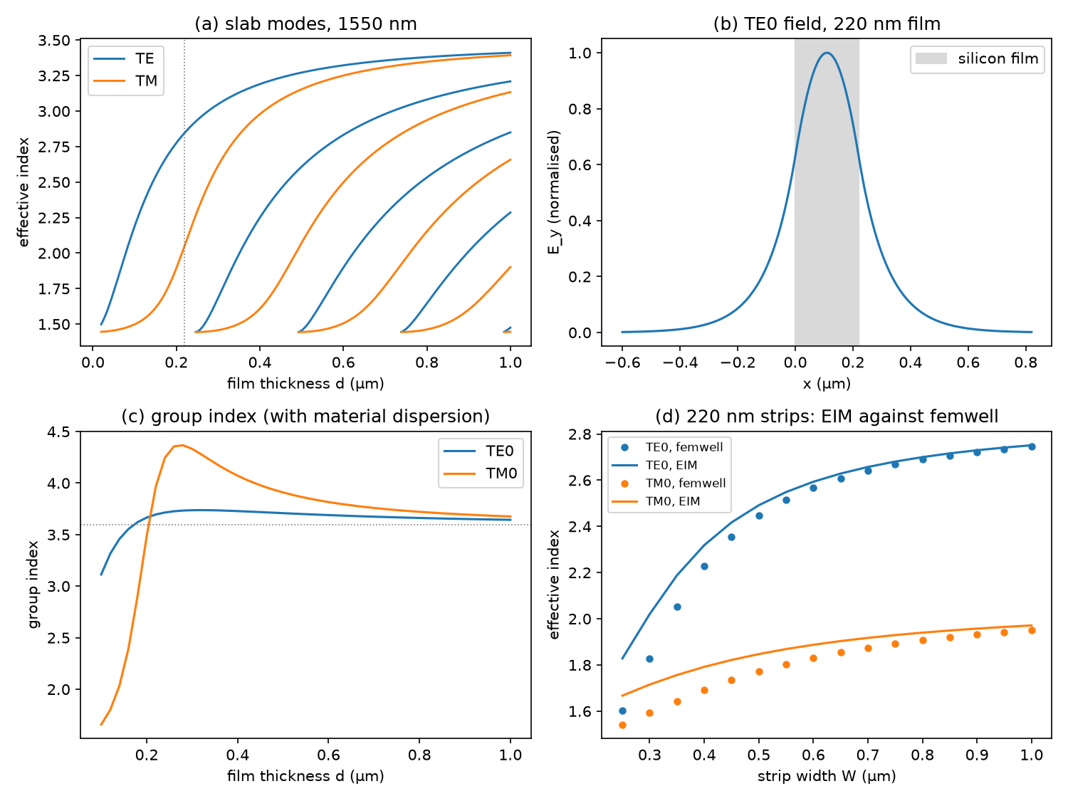
220 nm of silicon (\(n_1 = 3.476\)) in oxide (1.444) at 1550 nm has one TE mode, \(n_\mathrm{eff} = 2.8478\), and one TM mode, \(n_\mathrm{eff} = 2.0533\) (Worked Example 5.1). With an air cover instead of oxide, TE0 drops to 2.8309.
L1.2Field, decay length and confinement
Inside the film the TE field is a cosine, \(E_y = \cos(\kappa x - \phi_2)\), and outside it decays as \(e^{-\gamma\lvert x\rvert}\) from each interface. te_field builds it on a grid, and confinement sums \(\lvert E\rvert^2\) inside the film and divides by the total (Section 5.5). The script also finds the thickness at which a second TE mode appears, by bisection on the solver itself, and compares it with the formula \(d = \lambda/(2\sqrt{n_1^2 - n_2^2})\) of Section 5.4.
For the 220 nm film’s TE0 mode: \(1/\gamma = 101\) nm, \(\Gamma = 0.810\), and a ray angle of 55.0° from the normal. The film is single-mode below 245.1 nm, by the formula and by the solver alike.
L1.3Group index with material dispersion
The group index \(n_g = n_\mathrm{eff} - \lambda\,\mathrm{d}n_\mathrm{eff}/\mathrm{d}\lambda\) (Section 5.6) needs the effective index at neighbouring wavelengths, with the materials’ indices at those wavelengths too. n_si and n_ox are Sellmeier fits for silicon and fused silica; group_index takes a central difference over ±5 nm. Plot (c) of the figure shows TM0 with the higher group index at 220 nm: plot (a) shows why, since its effective index is still rising steeply with thickness there, and so changes quickly with wavelength too.
TE0 \(n_g = 3.70\) and TM0 \(n_g = 3.96\), both above bulk silicon’s 3.59.
L1.4The effective-index method
A 500 × 220 nm strip has no closed-form modes. The effective-index method (Section 6.2) approximates it with two slab problems, and eim does exactly that:
- Solve the vertical slab of the core (220 nm) for \(n_\mathrm{I}\), and the slab beside it for \(n_\mathrm{II}\): just the cladding for a strip, or the thin remaining film for a rib.
- Solve a lateral slab of width \(W\) with core \(n_\mathrm{I}\) and claddings \(n_\mathrm{II}\), with the other polarisation’s boundary conditions. A TE-like mode’s electric field is normal to the side walls, so this slab is solved as TM.
The script compares the result with femwell’s full vectorial solutions, the numbers behind Table 6.1, which it carries as a small table (FEMWELL_TE0, FEMWELL_TM0).
For the 500 × 220 nm strip, the EIM gives TE0 \(n_\mathrm{eff} = 2.491\) against femwell’s 2.446, and TM0 1.847 against 1.771. It predicts TE1 from a width of 316 nm; femwell finds it between 400 and 450 nm. Its group index is 4.02 against 4.18. For a rib with a 90 nm slab it gives 2.600 against femwell’s 2.568. Its error shrinks from +0.226 at 250 nm width to +0.005 at 1 µm.
The EIM always overestimates here, for the two reasons given in Section 6.2: the field does not separate into a vertical and a lateral profile near the corners, and the lateral slab it builds, with a core index of 2.85 against oxide, has more contrast than the real strip. It does best for wide guides and for ribs, where the lateral contrast is lower.
Exercises
- Silicon nitride. Repeat Checkpoint A for 400 nm of silicon nitride (\(n = 1.996\)) in oxide. How many modes, and what is its single-mode thickness?
- The O band. Use
n_si(1.31)andn_ox(1.31)to solve the 220 nm film at 1310 nm. Is it still single-mode? - Thin and thick films. Find \(\Gamma\) and \(1/\gamma\) for 150, 300 and 500 nm films. Which would you choose for an evanescent sensor (Chapter 34), and which for low leakage through a thin buried oxide (Section 7.4)?
- Air cover. For the air-clad film of Checkpoint A, how far does the field reach into the air, and into the oxide below?
- Ribs. Compare
eim(w, 0.22, 0.09)with the strip for widths of 400, 500 and 800 nm, and find the rib’s TE1 cut-off withfirst_width_with. Why does the rib stay single-mode to a wider width?
Answers
- One TE mode (\(n_\mathrm{eff} = 1.743\)) and one TM mode (1.642); single-mode below 562 nm. The low contrast makes the mode large and weakly confined, which is why nitride waveguides are thicker and wider than silicon ones.
- No. With \(n_\mathrm{Si} = 3.500\) and \(n_\mathrm{ox} = 1.447\) the limit is 205.5 nm, so 220 nm also guides TE1 (\(n_\mathrm{eff} = 1.483\)) and TM1 (1.448). TE0 rises to 2.988. TE1 is only 0.036 above the oxide, so it is very weakly guided.
- \(\Gamma\) = 0.655, 0.894 and 0.965, and \(1/\gamma\) = 118, 92 and 84 nm (0.810 and 101 nm at 220 nm). A thin film puts more light in the cladding: better for sensing, worse for substrate leakage and for scattering at rough surfaces.
- 93 nm into air and 101 nm into the oxide: the larger contrast with air pulls the field in more tightly on that side.
- Strip against rib: 2.319 and 2.514 at 400 nm, 2.491 and 2.600 at 500 nm, 2.700 and 2.729 at 800 nm. The 90 nm slab gives \(n_\mathrm{II} = 2.103\) instead of 1.444, so the lateral contrast is lower and TE1 appears only from 404 nm, against 316 nm for the strip in the same EIM.
Going further
- Lab 2 replaces the EIM with femwell, a full vectorial finite-element solver, and adds loss.
- The slab and EIM demos of Chapters 5 and 6 run the same equations in your browser.
- Add a TM field function: \(H_y\) has the same form, but its derivative is continuous only after dividing by \(n^2\).