Chapter 1Why Integrated Photonics?
Electronics moves information with charge, photonics moves it with light, and integration puts thousands of optical components on one chip.
- compare optical and electrical interconnects by loss, bandwidth and energy per bit;
- name the main applications of photonic integrated circuits and what each one demands;
- map the building blocks of electronics onto their photonic counterparts, and see where the analogy breaks;
- explain why silicon is the workhorse platform and what it cannot do on its own;
- work in dBm and dB and add up an optical power budget;
- read the targets of the reference link that runs through this tutorial.
When does light beat copper, and what does a photonic chip need to do it?
1.1Light versus charge
A copper trace is a transmission line, and its loss grows with frequency: the current crowds into a skin a few micrometres thick at gigahertz frequencies, and the laminate around it absorbs more energy each cycle. A trace on a printed circuit board loses roughly a decibel per centimetre at tens of gigahertz, depending on the laminate, so a 100 Gb/s electrical lane can cross a board but not a room without equalisation, retimers and the power they burn.
An optical fibre has none of these problems. Its loss, about 0.2 dB per kilometre at 1550 nm, does not depend on how fast the light is modulated, because the modulation is a tiny fraction of the optical carrier frequency of about 193 THz. The C band alone, 1530–1565 nm, spans about 4.4 THz of spectrum, and wavelength-division multiplexing (WDM) puts many independent channels into it, on the same fibre, without interference between them.
The price of light is the conversion. Every optical link needs a light source, a modulator to write the data, and a detector to read it, and each of these costs energy, area and decibels. Optics wins when the distance is long enough, or the bandwidth high enough, that the fixed cost of conversion is smaller than the growing cost of pushing electrons through copper. Over the last two decades that crossover has moved from kilometres (telecom) to metres (data-centre racks) and is now moving to millimetres, with optics placed beside the switch or accelerator chip itself.
Table 1.1. Loss per unit length of some interconnects. Typical values; the copper figure depends strongly on frequency and laminate.
| Medium | Typical loss | Depends on the data rate? |
|---|---|---|
| PCB copper trace, tens of GHz | of the order of 1 dB/cm | yes, rises with frequency |
| Standard single-mode fibre, 1550 nm | 0.2 dB/km | no |
| Standard single-mode fibre, 1310 nm | 0.35 dB/km | no |
| Multimode fibre, 850 nm | about 3 dB/km | no (but modal dispersion limits reach) |
| Silicon strip waveguide, 1550 nm | 1–3 dB/cm | no |
| Low-loss silicon nitride waveguide | down to about 0.1 dB/m [31] | no |
The last two rows show that on-chip waveguides are not long-distance media: a silicon waveguide loses more per metre than copper does at low frequencies. A photonic chip’s job is to generate, shape and process light over millimetres and to hand it to a fibre for the long haul.
Electronics and photonics side by side
It helps to map the building blocks of an electronic circuit onto their photonic counterparts (Table 1.2). The analogy is useful for orientation, and it breaks in instructive places.
Table 1.2. Electronic and photonic circuits compared.
| Electronic circuit | Photonic integrated circuit | |
|---|---|---|
| Carrier | electrons and holes | photons |
| Source | supply, clock | laser |
| Interconnect | metal wire, transmission line | waveguide, fibre |
| What sets propagation | impedance, RC, LC | effective index, group index, loss |
| Passive elements | R, L, C, transformers, filters | couplers, splitters, interferometers, rings, gratings |
| Active elements | transistors | modulators, detectors, amplifiers, lasers |
| Typical feature size | tens of nanometres | the wavelength in the material, about 0.2–1 µm |
| Parallelism | many wires | many wavelengths in one waveguide |
Three differences matter most. First, photonic circuits are linear in the optical field and work by interference, so phase is as important as amplitude: a path-length error of a fraction of a wavelength changes the output completely. Second, photons barely interact with each other, which is why many wavelengths can share a waveguide, and also why there is no compact photonic transistor or memory; photonics carries and transforms information, electronics decides and stores. Third, optical components are set by the wavelength, so they are hundreds of times larger than transistors: a photonic chip with thousands of components is large-scale integration for photonics.
1.2Applications
Photonic integrated circuits (PICs) are now in several markets, each pulling the design in a different direction.
- Data-centre transceivers and AI clusters. Pluggable modules convert electrical lanes to light over hundreds of metres to a few kilometres of fibre at 400 Gb/s, 800 Gb/s and beyond. Clusters of AI accelerators need far more bandwidth between chips than copper can deliver at acceptable power, which is driving optics into the package (co-packaged optics, Chapter 17).
- Coherent telecom. Long-haul and metro links encode data in the amplitude and phase of light in two polarisations and recover it with a local oscillator and digital signal processing. They need low-loss IQ modulators and narrow-linewidth tunable lasers (Chapters 20 and 26).
- LiDAR and free-space beam steering. Frequency-modulated continuous-wave (FMCW) LiDAR measures distance and velocity from the beat between transmitted and received light; optical phased arrays steer the beam without moving parts (Chapter 34).
- Sensing. The evanescent field of a waveguide resonator responds to molecules binding at its surface, giving label-free biosensors; the same idea detects gases and measures rotation and strain.
- Quantum photonics. Photon-pair sources, large interferometer meshes and single-photon detectors on a chip are a route to quantum communication and computing.
- Photonic computing. Meshes of interferometers perform matrix multiplication at the speed of light, with the electronics around them as the bottleneck.
The roadmap by Shekhar and co-authors reviews where silicon photonics stands in each of these [28]. In all of them the same few building blocks recur: waveguides, couplers, interferometers, resonators, modulators, detectors and lasers. That is why this tutorial is organised by building block, and only returns to systems in Part VIII.
1.3Why silicon, and why not only silicon
Silicon photonics started from a simple observation: the silicon-on-insulator (SOI) wafers used for some CMOS processes also make excellent optical waveguides [7, 30]. A thin silicon film (most often 220 nm) sits on a buried oxide (BOX) 2–3 µm thick. Silicon is transparent at the telecom wavelengths, above about 1.1 µm, and its index of 3.48 against 1.44 for silica gives a very strong index contrast. Light can then be confined in a strip of silicon only 500 nm wide and turned around bends a few micrometres in radius, so complex circuits fit on a few square millimetres.
The decisive advantage is manufacturing. Silicon photonics uses the lithography, etching, implantation and metallisation tools of the CMOS industry, on 200 mm and 300 mm wafers, with the yield and statistics of that industry. Germanium, already used in CMOS for strain engineering, makes photodetectors; doped junctions make modulators; metal heaters make tuners. Foundries offer this as a multi-project wafer (MPW) service with a process design kit, so a designer without a fab can tape out a chip (Chapters 29 and 30).
Silicon has five weaknesses, and each one shapes the rest of this tutorial:
- No efficient light emission. Silicon has an indirect bandgap, so electrons and holes recombine through phonons and heat rather than light. The laser has to be brought in from another material (Chapters 22 and 27).
- No linear electro-optic effect. Silicon’s crystal is centrosymmetric, so it has no Pockels effect. Its modulators move free carriers instead, which costs loss and limits linearity (Chapter 19).
- Two-photon absorption. At 1550 nm the photon energy is 0.80 eV, and two photons together exceed silicon’s 1.12 eV bandgap, so high intensities are absorbed (Chapter 7).
- Temperature sensitivity. Silicon’s index changes by about 1.8 × 10⁻⁴ per kelvin, so a silicon ring resonator drifts by about 80 pm/K and needs active control (Chapter 18).
- Sensitivity to fabrication. The strong confinement that makes devices small also makes them sensitive to nanometre changes in width and thickness (Chapter 29).
These weaknesses are why other materials have joined silicon: silicon nitride for low loss and wide transparency, thin-film lithium niobate and barium titanate for fast, efficient modulation, and indium phosphide and other III–V semiconductors for gain. Chapter 4 compares them.
1.4Anatomy of a photonic integrated circuit
Figure 1.1 shows the blocks of an optical link and the chapters that cover each. A laser provides a continuous optical carrier. A modulator writes data onto it by changing its amplitude or phase. Passive devices route, split, combine and filter the light: waveguides, couplers, interferometers, ring resonators and gratings. A coupler hands the light to a fibre, and on the far side another coupler brings it onto the receiving chip, where a demultiplexer separates the wavelengths and photodetectors turn each back into a current for the electronics.
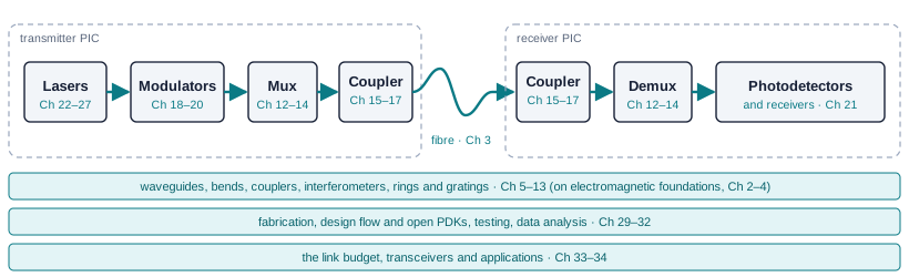
The electronics around the PIC (laser drivers, modulator drivers, transimpedance amplifiers, control loops for heaters) are as important as the optics. They can sit on the same die (monolithic integration, as in silicon-photonic processes that keep the CMOS transistors [55]), on a separate die placed beside the PIC on an interposer (2.5D), or stacked on top of it with dense bonds (3D). The choice is a trade between the best transistors, the best photonics, and the parasitics of the connection between them.
1.5Optical power and decibels
Optical powers span many orders of magnitude, from tens of milliwatts out of a laser to microwatts at a receiver, so they are quoted on a logarithmic scale. Power in dBm is power relative to one milliwatt; a gain or loss in dB is a ratio:
So 1 mW is 0 dBm, 10 mW is +10 dBm and 1 µW is −30 dBm; 3 dB is a factor of two and 10 dB a factor of ten. Because losses multiply, their decibels add, and a link budget becomes a subtraction. Two warnings: dBm describes a power and dB a ratio, so adding two dBm values is meaningless; and power ratios use 10 log₁₀, field ratios 20 log₁₀.
Two more quantities describe a modulated signal. The extinction ratio ER is the ratio of the power in a “one” to the power in a “zero”, \(P_1/P_0\), usually in dB. The optical modulation amplitude OMA is their difference, \(P_1 - P_0\), and it is what a receiver actually detects. For an average power \(\bar P = (P_1 + P_0)/2\) and a linear extinction ratio \(r = P_1/P_0\),
\[\mathrm{OMA} = 2\bar P\,\frac{r - 1}{r + 1}.\]A modulator with only 4 dB of extinction (\(r = 2.5\)) turns an average power into an OMA of only 0.86 times that power; a perfect one (\(r \to \infty\)) gives twice the average.
Take one wavelength of the reference link (Table 1.3), with first-guess losses. The laser puts +10 dBm (10 mW) into the transmitter waveguide. The ring modulator costs 3 dB at its operating point, the three other rings on the bus and the routing 0.8 dB, a grating coupler 3 dB, 2 km of fibre 0.4 dB plus 1 dB for two connectors, the receiving grating coupler 3 dB, and the demultiplexing ring and routing 1.5 dB:
\[P_\mathrm{rx} = 10 - (3 + 0.8 + 3 + 1.4 + 3 + 1.5) = 10 - 12.7 = -2.7\ \mathrm{dBm} \approx 0.54\ \mathrm{mW}.\]If the receiver needs −12 dBm average power at 50 Gb/s for the target error rate (Chapter 21 derives such a number), the margin is −2.7 − (−12) = 9.3 dB. That is plenty: most of it will be spent on penalties (extinction ratio, crosstalk, temperature drift, ageing), and what is left can be traded for a weaker laser.
The margin is not free energy to waste. At a wall-plug efficiency of 15 %, a laser delivering 10 mW draws about 67 mW; at 50 Gb/s that is 1.3 pJ for every bit, from the laser alone. Every 3 dB of margin given back halves it.
Try it. Change the losses and the laser power, and watch the margin and the laser’s share of the energy per bit.
The fibre couplers usually dominate a short link’s budget: two grating couplers at 3 dB each cost more than kilometres of fibre. That is why Part IV is devoted to coupling, and why every decibel saved there can be returned as laser power and energy per bit.
1.6The two running examples
Your first chip. The labs build a passive chip in 220 nm SOI at 1550 nm, with grating couplers on a 127 µm pitch for a fibre array, of the kind fabricated in the SiEPIC openEBL runs [14]. It carries the classic test structures: waveguide cut-backs to measure loss, Mach–Zehnder interferometers to measure the group index, ring resonators and Bragg gratings. You lay it out with open tools (Chapter 30), and Chapter 32 analyses measured data from chips like it, so that the tutorial covers a whole design–fabrication–test cycle.
The reference link. The system thread of the tutorial is a four-wavelength WDM link (Figure 1.2): four lasers, four ring modulators on one bus, a grating coupler into 2 km of single-mode fibre, and on the receiving chip four drop rings that separate the wavelengths onto germanium photodiodes. Ring modulators double as the multiplexer, which keeps the transmitter compact; the price is that every ring must be held on its wavelength by a heater and a control loop. Table 1.3 lists its draft targets, and the chapter that sets or meets each.
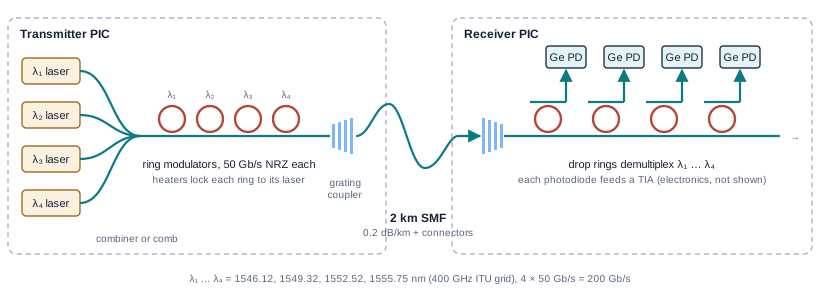
Table 1.3. Draft targets of the reference link. Set here, checked block by block, and closed in Chapter 33.
| Quantity | Draft target | Set or met in |
|---|---|---|
| Channels | 4 wavelengths on the 400 GHz ITU grid: 1546.12, 1549.32, 1552.52, 1555.75 nm [56] | Ch 12, 14 |
| Modulation and rate | NRZ, 50 Gb/s per channel, 200 Gb/s in total | Ch 20, 21 |
| Reach | 2 km of standard single-mode fibre, two connectors | Ch 3, 34 |
| Bit-error ratio | below 10⁻¹² without forward error correction | Ch 21, 34 |
| Laser | ≥ +10 dBm per wavelength in the waveguide; side-mode suppression ≥ 35 dB | Ch 24–27 |
| Ring modulator | extinction ≥ 4 dB with ≤ 2 V peak-to-peak drive; insertion loss ≤ 3 dB | Ch 12, 19, 20 |
| Fibre couplers | ≤ 3 dB each, 1 dB bandwidth covering all four channels | Ch 15–17 |
| Demultiplexer | crosstalk from neighbouring channels ≤ −20 dB; drop loss ≤ 1 dB | Ch 12, 14 |
| Receiver | sensitivity ≤ −12 dBm average power at 50 Gb/s | Ch 21 |
| Temperature | rings held on their channels from 20 to 70 °C | Ch 18 |
| Link margin | ≥ 3 dB after all penalties | Ch 33 |
| Energy | ≤ 5 pJ/bit for the whole link, including laser wall-plug power, drivers, receivers and heaters | Ch 33 |
The 400 GHz spacing (about 3.2 nm) is wide enough that ring filters with a free spectral range above the 9.6 nm span of the four channels separate them cleanly, and it leaves room for the thermal drift that the heaters must correct. At 80 pm/K, a 50 K temperature change moves a silicon ring by 4 nm, more than one channel spacing: thermal control is not optional.
Four wavelengths at 1546.12–1555.75 nm, 4 × 50 Gb/s NRZ over 2 km of single-mode fibre at a bit-error ratio below 10⁻¹², with at least 3 dB of margin and no more than 5 pJ/bit for the whole link.
1.7How to use this tutorial
The preface suggests reading paths for physics-first readers, chip designers, laser specialists and test engineers, and the course map shows every chapter on one page. Each chapter has the same parts: what you will learn, a design question, derivations with key equations, worked examples with real numbers, what this means for your design boxes, interactive demos, links to free simulations by others, reading, and key takeaways. The 3D gallery shows devices from open process design kits.
A few conventions hold throughout. Wavelengths are in vacuum unless stated otherwise; lengths on chips are in micrometres and nanometres. Time-harmonic fields vary as \(e^{j(\omega t - \beta z)}\), the engineering convention; many physics texts use \(e^{-i(\omega t - kz)}\), which flips the sign of every imaginary part (Chapter 2). “TE” and “TM” for waveguide modes mean the electric field mostly in the plane of the chip or mostly normal to it (Chapter 5).
- VM-Lab game: DataBytes Inc., a game about running a data centre, from the MIT Virtual Manufacturing Lab and AIM Photonics Academy [11].
Reading
- [28] Sudip Shekhar, Wim Bogaerts, Lukas Chrostowski, John E. Bowers, Michael Hochberg, Richard Soref and Bhavin J. Shastri. “Roadmapping the next generation of silicon photonics.” Nature Communications, 15:751, 2024. Open access.
- [30] Michael Hochberg, Nicholas C. Harris, Ran Ding et al. “Silicon photonics: the next fabless semiconductor industry.” IEEE Solid-State Circuits Magazine, 5(1):48–58, 2013.
- [29] Shawn Yohanes Siew et al. “Review of silicon photonics technology and platform development.” Journal of Lightwave Technology, 39(13):4374–4389, 2021. Open access.
- [1] Lukas Chrostowski and Michael Hochberg. Silicon Photonics Design: From Devices to Systems. Cambridge University Press, 2015. https://www.cambridge.org/core/books/silicon-photonics-design/BF3CF13E8542BCE67FD2BBC7104ECEAB
- [7] Graham T. Reed and Andrew P. Knights. Silicon Photonics: An Introduction. Wiley, 2004.
- Copper loss rises with frequency; fibre loss (0.2 dB/km at 1550 nm) does not. Optics wins once distance or bandwidth makes the fixed cost of electro-optic conversion worth paying, and that crossover is moving into the package.
- Photonic circuits are linear, interferometric and wavelength-parallel; they have no compact equivalent of the transistor or memory.
- Silicon offers CMOS manufacturing and strong confinement, but no efficient laser, no Pockels effect, two-photon absorption at 1550 nm and a large thermo-optic coefficient. Other materials fill these gaps.
- In decibels a link budget is a subtraction; the fibre couplers usually dominate a short link, and margin can be traded for laser power and energy.
- The reference link (4 × 50 Gb/s, 2 km, BER < 10⁻¹², ≤ 5 pJ/bit) and a first openEBL-style chip run through the rest of the tutorial.