Lab 10 · Lasers and linksLaser Rate Equations in Python
Solve the rate equations of the Chapter 24 laser with your own Runge–Kutta integrator, and reproduce its threshold, L–I curve, switch-on, modulation bandwidth, temperature dependence and noise from Chapters 24 and 25.
- compute the threshold of a cleaved Fabry–Pérot laser from its cavity: mirror loss, threshold gain, carrier density and current;
- trace the steady-state L–I curve, including the spontaneous emission below threshold;
- integrate the switch-on transient with a fourth-order Runge–Kutta method, and measure the turn-on delay and the relaxation oscillations;
- compute the small-signal modulation response against bias, and check the formula by linearising the rate equations numerically;
- follow the threshold with temperature, and compute the intensity noise and the linewidth.
What you need
- Chapter 24 (Sections 24.1 to 24.6) and Chapter 25 (Sections 25.1, 25.3 and 25.4).
- Python 3.11 or newer with NumPy and Matplotlib:
pip install numpy matplotlib. No ODE library: the script brings its own integrator. - The script
lab10_rate_equations.py(also in the repository’slabs/folder). - About two hours, including the exercises.
Run it from a terminal in the folder where you saved it:
python lab10_rate_equations.py
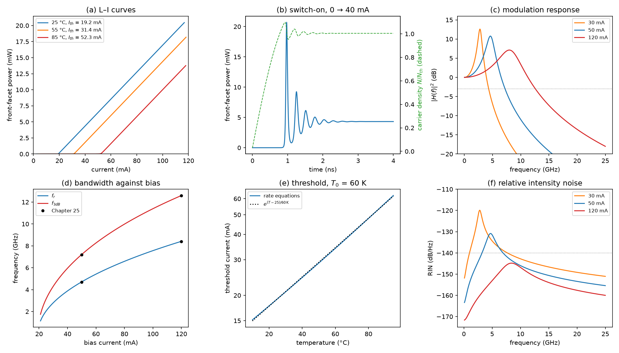
It prints a checkpoint for each part below, with the value from the chapter beside it, and saves the figure lab10_rate_equations.png in a few seconds. Read each part, then the matching function in the script; change things and run it again. Inside, the script works in the chapters’ units, centimetres and seconds; it prints milliamperes, milliwatts, nanoseconds and gigahertz.
The laser is the one of Worked Example 24.1 and of the demos in Chapters 24 and 25: an InGaAsP active region 2 µm wide and 50 nm thick in a 400 µm cavity with cleaved facets, \(n_g = 3.6\), \(\Gamma = 0.06\), \(\eta_i = 0.8\), \(\alpha_i = 15\) cm⁻¹, gain \(g(N) = g_0\ln(N/N_\mathrm{tr})\) with \(g_0 = 1500\) cm⁻¹ and \(N_\mathrm{tr} = 2\times10^{18}\) cm⁻³, gain compression \(\varepsilon = 2\times10^{-17}\) cm³, \(\beta = 10^{-4}\), and the recombination coefficients of Chapter 23. They are the constants at the top of the script.
L10.1The cavity and the threshold
The threshold condition of Section 24.2, \(\Gamma g_\mathrm{th} = \alpha_i + \alpha_m\), fixes the gain the laser needs; the gain model turns it into a carrier density \(N_\mathrm{th} = N_\mathrm{tr}\,e^{g_\mathrm{th}/g_0}\), and the recombination at that density sets the current. The function laser follows the chapter line by line:
    am = math.log(1 / (R1 * R2)) / (2 * L)                # mirror loss (1/cm)
    tp = 1 / (VG * (ALPHA_I + am))                        # photon lifetime (s)
    Ntr = NTR0 * math.exp((T - 25) / T0N)                 # transparency density: rises with temperature
    gth = (ALPHA_I + am) / GAMMA                          # threshold gain: Gamma g_th = alpha_i + alpha_m
    Nth = Ntr * math.exp(gth / G0)                        # the carrier density that gives it
    Ith = Q * V / ETA_I * recomb(Nth)                     # threshold current (A)
    eta_d = ETA_I * am / (ALPHA_I + am)                   # differential quantum efficiency, both facets
    F1 = (1 - R1) / ((1 - R1) + math.sqrt(R1 / R2) * (1 - R2))   # share of the output leaving the front facet
\(\eta_d\) counts the photons that leave through both mirrors. With equal facets each takes half (\(F_1 = 0.5\)); with unequal ones the front facet’s share is \(F_1 = (1 - R_1)/[(1 - R_1) + \sqrt{R_1/R_2}\,(1 - R_2)]\). The slope per facet is \(\eta_dF_1h\nu/q\), with \(h\nu/q = 0.80\) V at 1550 nm.
Mode spacing 0.83 nm, \(\alpha_m = 28.5\) cm⁻¹ and \(\tau_p = 2.76\) ps (Chapters 24 and 25: the same). \(g_\mathrm{th} = 725\) cm⁻¹, \(N_\mathrm{th} = 3.24\times10^{18}\) cm⁻³ and \(R(N_\mathrm{th}) = 2.40\times10^{27}\) cm⁻³ s⁻¹ give \(I_\mathrm{th} = 19.2\) mA (Worked Example 24.1: 725 cm⁻¹, 3.24 × 10¹⁸, 2.4 × 10²⁷ and 19 mA; the demo reads 19.2 mA). \(\eta_d = 0.524\) and the slope is 0.210 W/A per facet (Chapter 24: 0.52 and 0.21 W/A).
L10.2The steady-state L–I curve
Solving the rate equations for \(N\) and \(S\) at each current means solving two nonlinear equations. li_curve turns the problem round instead, as the Chapter 24 demo does: it chooses the carrier density, closer and closer to its clamped value \(N_\mathrm{th}\), and asks what photon density and what current go with it. With \(\mathrm{d}S/\mathrm{d}t = 0\), the photons in the mode are the spontaneous seed amplified by a gain that falls just short of the loss; with \(\mathrm{d}N/\mathrm{d}t = 0\), the current replaces every carrier lost:
    x = 10 ** (-0.2 - 7 * np.arange(n + 1) / n)          # 1 - N/N_th, from 0.63 down to 6e-8
    N = lz["Nth"] * (1 - x)
    g = G0 * np.log(N / lz["Ntr"])
    S = GAMMA * BETA * B_RAD * N**2 / (1 / lz["tp"] - GAMMA * VG * g)
    I = Q * lz["V"] / ETA_I * (recomb(N) + VG * g * S)
As \(N\) approaches \(N_\mathrm{th}\) the denominator of S goes to zero and the photon density grows without limit, while the current only creeps up: that is the clamping of Section 24.2, seen from the inside. Gain compression is left out here, as in the demo; the transient of the next part includes it.
At 50 mA the front facet emits 6.45 mW, the same as the straight line \(\eta_dF_1(h\nu/q)(I - I_\mathrm{th})\) (Chapter 24: about 6.5 mW). With a 0.85 V diode drop and 5 Ω, the electrical input is 55 mW and the wall-plug efficiency of both facets together is 23.5 % (Chapter 24: about 23 %). At threshold each facet already emits 28 µW, the spontaneous emission that falls into the mode.
L10.3Switch-on with a Runge–Kutta integrator
The function rates returns \(\mathrm{d}N/\mathrm{d}t\) and \(\mathrm{d}S/\mathrm{d}t\) from the key equations of Section 24.3, gain compression included. To follow them in time, the script writes the classic fourth-order Runge–Kutta method: four slopes per step, at the start, twice at the midpoint and at the end, averaged with weights 1, 2, 2, 1. Its error per step falls as the fifth power of the step.
def rk4(f, y0, dt, n_steps):
    ys = np.empty((n_steps + 1, len(y0)))
    y = np.array(y0, dtype=float)
    for k in range(n_steps + 1):
        ys[k] = y
        k1 = f(y)
        k2 = f(y + dt / 2 * k1)
        k3 = f(y + dt / 2 * k2)
        k4 = f(y + dt * k3)
        y = y + dt / 6 * (k1 + 2 * k2 + 2 * k3 + k4)
    return ys
The fastest process is the escape of photons, \(\tau_p = 2.76\) ps, so turn_on takes steps of 0.5 ps: 8000 steps for 4 ns. Like the demo, it starts from a nearly empty laser (\(N = 10^{17}\) cm⁻³, \(S = 1\) cm⁻³) and steps the current to 40 mA at \(t = 0\). Three things happen in turn (plot (b) of the figure). The carriers build up while the light stays dark. Once \(N\) passes \(N_\mathrm{th}\) the photons grow exponentially from the spontaneous seed; by the time they are numerous the carriers have overshot, so the first pulse is far above the final power. Then photons and carriers trade energy back and forth: the relaxation oscillations, which die away in about a nanosecond. peaks finds the maxima, each refined with a parabola through its neighbours, and the ringing frequency is the inverse of their mean spacing.
The carrier lifetime at threshold, \(N_\mathrm{th}/R(N_\mathrm{th})\), is 1.35 ns, and \(\tau_n\ln[I/(I - I_\mathrm{th})] = 0.88\) ns at 40 mA (Section 24.6: 1.35 ns and 0.9 ns). In the simulation the carriers reach \(N_\mathrm{th}\) at 0.77 ns, the light passes half its final power at 0.92 ns, and the first peak, 20.7 mW, comes at 0.97 ns. The ringing is at 3.83 GHz, and the output settles at 4.32 mW (the Chapter 24 demo reads \(f_r\) = 3.9 GHz at 40 mA).
The formula assumes a constant carrier lifetime. Since \(R(N)\) grows faster than linearly, carriers at low density live longer than 1.35 ns, so they build up faster and reach \(N_\mathrm{th}\) sooner: 0.77 ns. The light needs another 0.15 ns to grow from the spontaneous seed, and the two errors nearly cancel. The final 4.32 mW is a little below the 4.36 mW of the L–I curve at 40 mA because gain compression, included here, holds \(N\) slightly above \(N_\mathrm{th}\), where more carriers recombine.
L10.4Small-signal modulation response
Add a small sinusoid to the bias current and the photon density responds like the damped oscillator of Section 25.1. small_signal computes its parameters as the Chapter 25 demo does: the photon density from the linear L–I curve, the differential gain \(a = g_0/N_\mathrm{th}\), \(\omega_r^2 = v_gaS/[\tau_p(1 + \varepsilon S)]\), the K-factor, and a damping \(\gamma = Kf_r^2 + \gamma_0\) whose floor \(\gamma_0\) is the inverse of the differential carrier lifetime \(\mathrm{d}N/\mathrm{d}R = 1/(A + 2BN + 3CN^2) = 0.59\) ns. f3db finds where \(\lvert H\rvert^2\) falls to one half, by bisection on a logarithmic frequency scale.
The formula is itself an approximation, so the script checks it. steady_state finds the operating point of the full rate equations, gain compression and spontaneous emission included, by Newton’s method; jacobian differentiates the rate equations numerically; and linearised solves the linear system they define:
    y = steady_state(I, lz)
    J = jacobian(y, I, lz)
    b = np.array([ETA_I / (Q * lz["V"]), 0.0])
    dS0 = np.linalg.solve(-J, b)[1]
    response = lambda f: abs(np.linalg.solve(2j * np.pi * f * np.eye(2) - J, b)[1] / dS0) ** 2
    ev = np.linalg.eigvals(J)
A small current \(\delta I\,e^{j\omega t}\) drives \((j\omega - J)\,\delta y = b\,\delta I\), where \(b\) is the carriers it injects per second. The two eigenvalues of \(J\) are \(-\gamma/2 \pm j\omega_d\): their real part is the damping, and \(\omega_d = \sqrt{\omega_r^2 - \gamma^2/4}\) is the frequency at which a disturbance rings, slightly below \(\omega_r\).
\(f_r\) = 4.72 GHz and \(f_\mathrm{3dB}\) = 7.22 GHz at 50 mA, and 8.41 and 12.60 GHz at 120 mA (Worked Example 25.1: 4.7 and 7.2 GHz, 8.4 and 12.6 GHz); 3.88 and 5.96 GHz at 40 mA. \(a = 4.63\times10^{-16}\) cm² and \(K\) = 314 ps, which caps the bandwidth at \(2\pi\sqrt{2}/K\) = 28.3 GHz (Chapter 25: 4.6 × 10⁻¹⁶ cm², 314 ps and about 28 GHz). Linearising the full equations gives \(f_r\) = 4.70 GHz, \(\gamma\) = 8.62 ns⁻¹ and \(f_\mathrm{3dB}\) = 7.20 GHz at 50 mA; at 40 mA, \(f_r\) = 3.88 GHz, \(\gamma\) = 6.40 ns⁻¹, ringing at \(f_d\) = 3.84 GHz, and \(f_\mathrm{3dB}\) = 5.95 GHz.
The formula and the full linearisation agree within 1 %. The linearised ringing frequency at 40 mA, 3.84 GHz, is also what the Runge–Kutta transient measured, 3.83 GHz: once the switch-on overshoot has decayed, the ringing is a small-signal oscillation. Plot (d) shows \(f_r\) growing as \(\sqrt{I - I_\mathrm{th}}\), and \(f_\mathrm{3dB}\) staying about 1.5 times \(f_r\) while the damping is light.
L10.5Temperature
The demo of Chapter 24 heats the laser by raising its transparency density, \(N_\mathrm{tr} \propto e^{(T - 25\,{}^\circ\mathrm{C})/T_{0N}}\) with \(T_{0N}\) = 143 K: a hotter laser needs more carriers for the same gain (Fermi smearing, Section 23.6). Every other quantity follows: \(N_\mathrm{th}\) grows with \(N_\mathrm{tr}\), and the threshold current with \(R(N_\mathrm{th})\). Why 143 K for a threshold \(T_0\) of 60 K? Near \(N_\mathrm{th}\) the recombination grows as a power of the density, \(R \propto N^p\) with \(p = \mathrm{d}\ln R/\mathrm{d}\ln N\), so \(I_\mathrm{th} \propto e^{p(T - 25\,{}^\circ\mathrm{C})/T_{0N}}\) and \(T_0 \approx T_{0N}/p\). The Auger term, the steepest, makes \(p\) grow with \(N\), so \(T_0\) falls slowly as the laser heats.
\(I_\mathrm{th}\) = 19.2, 31.4 and 52.3 mA at 25, 55 and 85 °C (Section 24.5: from 19 to 52 mA). Over the 60 K, \(T_0 = 60\ \mathrm{K}/\ln(52.3/19.2)\) = 59.9 K (Chapter 24: 60 K). At 25 °C, \(p\) = 2.29 and \(T_{0N}/p\) = 62 K. At 85 °C a 50 mA bias is below threshold: the front facet emits only 10 µW.
L10.6Intensity noise and linewidth
rin is the Chapter 25 demo’s simplified Langevin model: the spontaneous emission’s random kicks, filtered by the same response as the modulation, plus the shot-noise floor \(2h\nu/P\). It peaks at the relaxation oscillation and falls with power. linewidth is the key equation of Section 25.4 written per photon in the cavity:
def linewidth(ss, alpha=4.0):
    return ss["Rsp"] * (1 + alpha**2) / (4 * math.pi * ss["Np"])
\(R_\mathrm{sp} = v_g\Gamma g_\mathrm{th}n_{sp}\) is the rate at which spontaneous photons join the mode, and \(N_p\) the number of photons in it. With \(P_0 = N_ph\nu v_g\alpha_m/2\) per facet this is the chapter’s \(\Delta\nu = v_g^2h\nu\Gamma g_\mathrm{th}n_{sp}\alpha_m(1 + \alpha^2)/(8\pi P_0)\).
At 50 mA the RIN peaks at −130.9 dB/Hz at 4.7 GHz and falls to −163.4 dB/Hz at 100 MHz, near the shot-noise floor of −167.0 dB/Hz; at 120 mA the peak is −144.8 dB/Hz at 8.4 GHz. The linewidth at 50 mA, 6.45 mW per facet, is 2.08 MHz with \(\alpha = 4\) and 0.122 MHz with \(\alpha = 0\) (Section 25.4: 2.1 and 0.12 MHz at 6.5 mW).
The Chapter 25 reference link asks for RIN below about −140 dB/Hz. This laser’s noise meets that at low frequencies from about 25 mA, but its relaxation-oscillation peak stays above it until much higher currents (Exercise 4): one more reason the link uses continuous-wave lasers and external modulators.
Exercises
- A high-reflection rear facet. Use
laser(R2=0.9). What happens to \(\alpha_m\), the threshold and the front-facet slope? How much does the front facet emit at 50 mA? - The best cavity length. Scan
laser(L_um=L)from 100 to 1500 µm. Which length gives the lowest threshold, and why does the threshold rise on both sides? What happens to the slope? - Pre-bias. Run
turn_onat 15 mA for 30 ns (steps of 1 ps are fine), and use its last state asy0for a step to 40 mA. How long is the turn-on delay now? Compare with \(\tau_n\ln[(I - I_b)/(I - I_\mathrm{th})]\). - Bandwidth and noise targets. At what bias does \(f_\mathrm{3dB}\) reach 10 GHz? At what bias does the RIN peak fall below −140 dB/Hz? Use bisection on
small_signal, asf3dbdoes on frequency. - A hot laser. At 85 °C, what current gives the same 6.45 mW per facet as 50 mA does at 25 °C? What are \(f_r\), \(f_\mathrm{3dB}\), the linewidth and the wall-plug efficiency there, and why has the bandwidth fallen?
Answers
- \(\alpha_m\) falls from 28.5 to 15.6 cm⁻¹, the threshold from 19.2 to 13.9 mA, and \(\eta_d\) from 0.52 to 0.41. But 92 % of the light now leaves through the front facet, so its slope rises from 0.21 to 0.30 W/A, and it emits 10.8 mW at 50 mA instead of 6.45 mW.
- About 300 µm, with 18.4 mA (slope 0.23 W/A). A shorter cavity has less volume to pump but more mirror loss, so a higher \(N_\mathrm{th}\), and \(R(N)\) grows as roughly \(N^{2.3}\): 20.3 mA at 200 µm, where \(N_\mathrm{th} = 4.45\times10^{18}\) cm⁻³. A longer one needs less gain but has more volume: 26.9 mA at 800 µm. The slope falls with length, from 0.25 W/A at 200 µm to 0.16 W/A at 800 µm, as the useful mirror loss shrinks against the internal loss.
- 0.27 ns instead of 0.92 ns: at 15 mA the carriers already sit at \(0.90N_\mathrm{th}\). The formula gives 0.25 ns. Lasers for direct modulation are biased just below or above threshold for this reason.
- \(f_\mathrm{3dB}\) = 10 GHz at 80.2 mA (\(f_r\) = 6.6 GHz, 12.8 mW per facet). The RIN peak falls below −140 dB/Hz from 86.7 mA (\(f_r\) = 6.9 GHz, 14.1 mW per facet).
- 83.1 mA, against a threshold of 52.3 mA. \(f_r\) = 3.82 GHz and \(f_\mathrm{3dB}\) = 5.78 GHz, down from 4.72 and 7.22 GHz: the photon density is the same, but the differential gain \(g_0/N_\mathrm{th}\) has fallen from 4.63 to 3.04 × 10⁻¹⁶ cm² because \(N_\mathrm{th}\) grew by 1.52. The linewidth is unchanged in this model, 2.08 MHz, since it depends only on the photon number and the losses. The wall-plug efficiency drops from 23.5 % to 12.3 % (1.27 V at 83 mA).
Going further
- Lab 11 adds wavelength selection: two ring filters, a gain window and a tuning map.
- The laser demo of Chapter 24 and the dynamics demo of Chapter 25 run the same equations in your browser.
- Add self-heating: raise \(T\) by \(Z_\mathrm{th}(IV - P_\mathrm{out})\) with \(Z_\mathrm{th}\) = 80 K/W (Section 27.6), iterate to a steady state at each current, and watch the L–I curve roll over.
- Drive
rateswith a 10 Gb/s current pattern instead of a step and draw the eye diagram; add the chirp \(\Delta\nu = (\alpha/4\pi)(\mathrm{d}\ln P/\mathrm{d}t + \kappa P)\) of Section 25.2.