Lab 5 · SimulateBragg Gratings with Transfer Matrices
Build a grating from its index steps, multiply 2 × 2 matrices along it, and check the formulas of Chapter 13 against the result: the Bragg wavelength, tanh²(κL), the bandwidth, apodisation and the quarter-wave-shifted cavity.
- write the transfer matrices of an index step and of a uniform layer, and multiply them along a grating;
- check the Bragg wavelength, peak reflectivity and bandwidth against coupled-mode theory;
- find the photonic band gap from the matrix of a single period;
- apodise a grating and measure its side lobes;
- open a cavity with a quarter-wave shift and measure its Q.
What you need
- Chapter 13 (Sections 13.1 to 13.5).
- Python 3.11 or newer with NumPy and Matplotlib:
pip install numpy matplotlib. - The script
lab05_bragg.py(also in the repository’slabs/folder). - About an hour and a half, including the exercises.
Run it from a terminal in the folder where you saved it:
python lab05_bragg.py
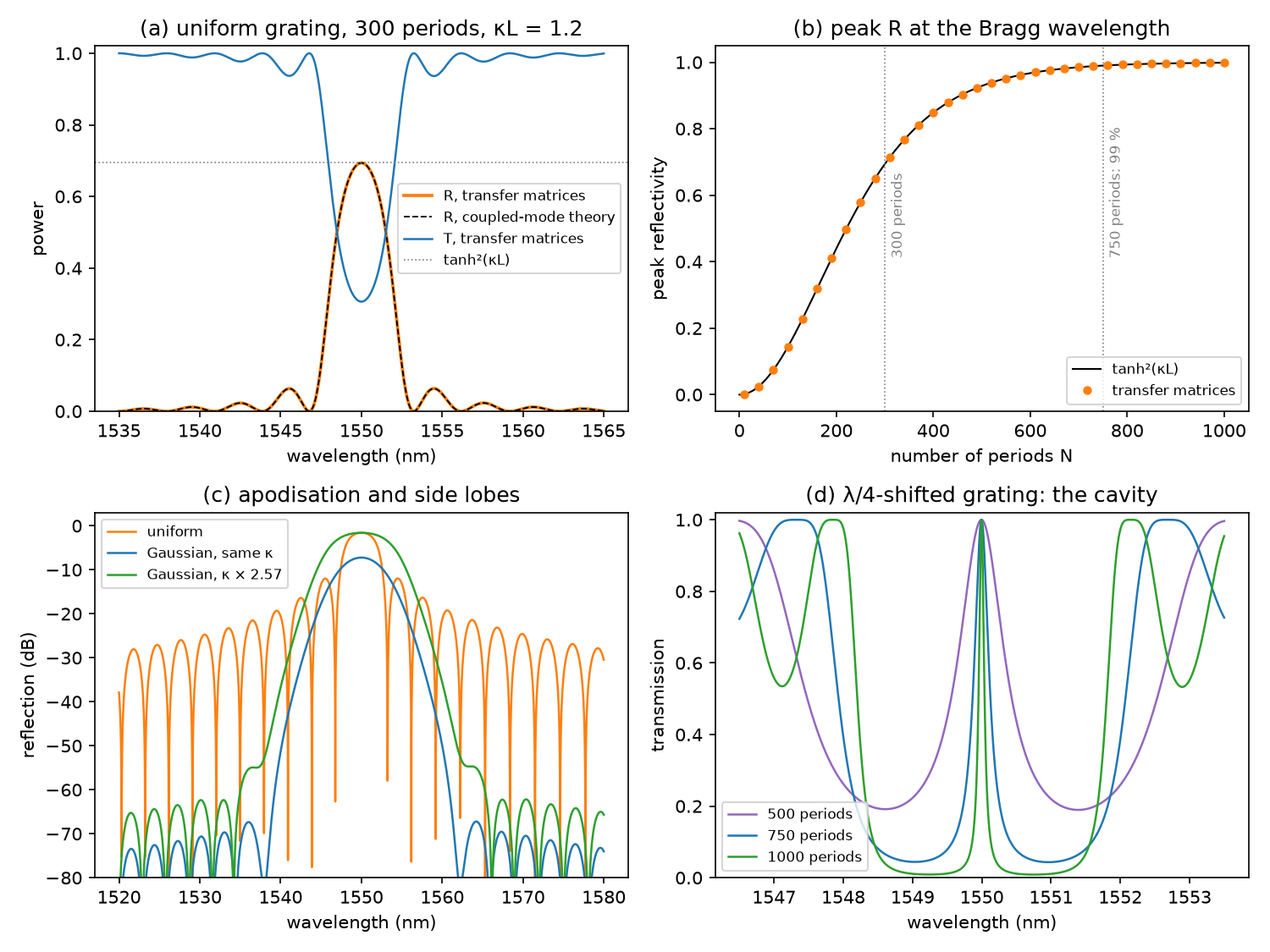
It prints a checkpoint for each part below, with the value from the chapter beside it, and saves the figure lab05_bragg.png in a few seconds. Read each part, then the matching function in the script; change things and run it again. All lengths are in micrometres.
The grating throughout is the one of Worked Examples 13.1 and 13.2, which is also the default of the chapter’s demo: a 500 × 220 nm silicon strip with \(n_\mathrm{eff} = 2.446\) and \(n_g = 4.18\) at 1550 nm, a period \(\Lambda = 316.8\) nm, \(\kappa = 12.6\) mm⁻¹ and 300 periods. The function n_eff lets the effective index fall with wavelength at the rate the group index sets, \(\mathrm{d}n_\mathrm{eff}/\mathrm{d}\lambda = -(n_g - n_\mathrm{eff})/\lambda\), as the demo does.
L5.1Index steps and transfer matrices
To the guided mode, a corrugated waveguide is a stack of layers half a period long, with effective indices \(n_\mathrm{eff} + \Delta n/2\) and \(n_\mathrm{eff} - \Delta n/2\). In each layer the field is a forward wave \(A\,e^{-j\beta z}\) plus a backward wave \(B\,e^{j\beta z}\), and two matrices describe everything that happens to them:
-
an index step from \(n_a\) to \(n_b\), from the continuity of the electric field (\(A + B\)) and of the magnetic field (\(n(A - B)\)):
\[\begin{pmatrix}A_a\\ B_a\end{pmatrix} = \frac{1}{2}\begin{pmatrix}1 + \rho & 1 - \rho\\ 1 - \rho & 1 + \rho\end{pmatrix}\begin{pmatrix}A_b\\ B_b\end{pmatrix}, \qquad \rho = \frac{n_b}{n_a};\] -
a uniform layer of length \(l\), the diagonal matrix with entries \(e^{j\beta l}\) and \(e^{-j\beta l}\), where \(\beta = 2\pi n/\lambda\).
Multiply them from input to output to get the grating’s matrix \(M\). Nothing enters from the far end, so the reflection and transmission are \(r = M_{21}/M_{11}\) and \(t = 1/M_{11}\). In the script:
def step(na, nb):
    p, m = 0.5 * (1 + nb / na), 0.5 * (1 - nb / na)
    return [[p, m], [m, p]]

def layer(n, length, lam):
    e = np.exp(2j * np.pi * n * length / lam)
    return [[e, 0 * e], [0 * e, 1 / e]]
Each entry is an array over wavelength, so one product computes a whole spectrum; mul writes the 2 × 2 product out by hand, which here is ten times faster than numpy.matmul. period_matrix multiplies the five matrices of one period, starting and ending in the unperturbed guide, and power raises it to the \(N\)th power by repeated squaring: 300 periods take 13 products.
Which \(\Delta n\) gives the chapter’s κ? A square wave of height \(\Delta n\) has a first Fourier component of amplitude \(2\Delta n/\pi\), and coupled-mode theory gives \(\kappa = \pi\,(2\Delta n/\pi)/\lambda = 2\Delta n/\lambda\). So 12.6 mm⁻¹ needs \(\Delta n = 0.00977\), 0.4 % of the effective index.
The period is 316.8 nm, and 300 periods make \(L = 95.1\) µm and \(\kappa L = 1.198\) (Worked Example 13.2: 95 µm and 1.2). The matrices give a peak reflectivity of 69.38 % at 1550.00 nm, the same as \(\tanh^2(\kappa L) = 69.38\) % (Chapter 13: 69 %), at the Bragg wavelength \(2n_\mathrm{eff}\Lambda = 1550.00\) nm. \(R + T = 1\) to within \(4\times10^{-13}\): the stack is lossless, and the matrices conserve energy.
L5.2Bandwidth, coupled-mode theory and the band gap
cmt_reflectivity is the closed-form result of coupled-mode theory for a uniform grating (Section 13.2),
Outside the stop-band \(s\) is imaginary, and \(r\) vanishes where \(\lvert s\rvert L = \pi\): these first nulls give the bandwidth formula of Section 13.2. first_nulls finds them in the matrix spectrum by walking from the peak to the first minimum on each side and refining it by golden-section search. To count the periods for 99 %, the script multiplies one more period at a time until \(R \geq 0.99\).
A grating without ends has a band gap instead of a reflection spectrum. Its modes are Bloch waves, \(e^{-jKz}\) times a function with the period of the grating, and the matrix \(P\) of one period fixes \(K\): \(\cos(K\Lambda) = (P_{11} + P_{22})/2\). Where the right-hand side exceeds 1 in magnitude, \(K\) is complex and no wave propagates. band_gap finds the edges of that range by bisection; its width should be \(\lambda^2\kappa/(\pi n_g)\), the long-grating limit of the bandwidth formula.
The first nulls are at 1546.77 and 1553.24 nm, a bandwidth of 6.47 nm, and the formula gives 6.47 nm (Worked Example 13.2: 6.5 nm). Over 1535–1565 nm the matrix spectrum differs from coupled-mode theory by at most 0.0007 in \(R\). 99 % reflection takes 750 periods, 238 µm (Chapter 13: 750 periods, 238 µm). The band gap of one period is 2.31 nm wide for 12.6 mm⁻¹, and 25.61 nm for the PDK’s 140 mm⁻¹, both equal to \(\lambda^2\kappa/(\pi n_g)\) (Chapter 13: about 25 nm).
The two methods agree so closely because the grating is weak. The matrices are exact for the stack of layers: they include every Fourier harmonic of the square wave and the exact reflection at each step. Coupled-mode theory keeps only the first harmonic, which is all that matters when \(\Delta n/n_\mathrm{eff}\) is 0.4 %. Exercise 2 tries a step ten times larger.
L5.3Apodisation
grating multiplies the periods one by one, each with its own index step, so the coupling can vary along the grating. gaussian gives the demo’s profile, \(\exp(-(z/0.22)^2)\) with \(z\) running from −0.5 to 0.5 along the grating, and side_lobe_db reports the strongest reflection beyond the first minimum on each side of the peak, in dB below the peak.
There are two fair comparisons. With the same maximum κ, the corrugation at the centre is the same. With the same peak reflectivity, κ must rise by 1/0.389 = 2.57, because the Gaussian averages 0.389 of its maximum and the peak depends on the average.
The uniform grating has a peak of 69.4 %, a full width at half maximum (FWHM) of 3.91 nm and its strongest side lobe at −10.4 dB. The Gaussian at the same κ: 18.9 %, 5.59 nm and −60.0 dB (Section 13.4: 19 % and 5.6 nm). The Gaussian with κ × 2.57: 69.4 %, 7.66 nm and −53.1 dB. A strong grating, κ = 100 mm⁻¹ (\(\kappa L = 9.5\)): 100.00 % and 19.1 nm uniform, 99.76 % and 18.7 nm apodised.
These are the two regimes of Section 13.4. A weak grating like the chapter’s has a reflection spectrum close to the Fourier transform of \(\kappa(z)\), so a smooth taper widens the main lobe, just as a window function widens a spectral peak, and the peak drops unless κ rises to compensate. A strong grating’s stop-band width is set by κ, and the apodised grating has less κ over most of its length, so its peak is only slightly lower and a little narrower. Either way, the side lobes fall by more than 40 dB.
L5.4A quarter-wave-shifted cavity
shifted builds the first half of the grating from high-then-low periods and the second half from low-then-high ones. The second half is moved by half a period, so the two low-index half-periods at the centre merge into one layer a full period long: half a wavelength in the guide at the Bragg wavelength. The two halves become mirrors facing each other across it (Section 13.5). cavity finds the transmission peak by golden-section search and its half-maximum points by bisection, and returns \(Q = \lambda/\mathrm{FWHM}\).
At 300 periods the transmission peak is there (100.0 % at 1549.993 nm), but each half has \(\kappa L = 0.6\) and reflects only 29 %, so the stop-band never falls below half and there is no FWHM to measure. With 500, 750 and 1000 periods (\(\kappa L\) = 2.0, 3.0 and 4.0) the transmission is 100.0 % at 1549.995–1549.996 nm, with an FWHM of 0.878, 0.258 and 0.088 nm: \(Q\) = 1766, 6008 and 17519.
The peak sits 4 pm short of 1550 nm because the central layer has the lower index, so it is a little less than half a wave long at \(\lambda_B\). \(Q\) grows by a factor of about 3 for each unit of \(\kappa L\): light leaves through the two mirrors, each with transmission \(1 - \tanh^2(\kappa L/2)\), which falls as \(e^{-\kappa L}\) once \(\kappa L\) exceeds 2 or so. This is the cavity of the λ/4-shifted DFB laser of Chapter 26, whose \(\kappa L\) is usually between 1 and 3.
Exercises
- The PDK’s period. The SiEPIC EBeam PDK rounds the period to 317 nm (Worked Example 13.1). Set
PERIOD = 0.317at the top of the script: where is the Bragg wavelength now, and why has it moved by less than \(2n_\mathrm{eff} \times 0.16\) nm? - A strong grating. With the PDK’s κ = 140 mm⁻¹ (\(\Delta n = 0.1085\)), how many periods reflect 99 %? Does \(\tanh^2(\kappa L)\) still hold with index steps of 4 %?
- Another window. Replace the Gaussian with a raised cosine, \(\sin^2(\pi u)\) with \(u\) running from 0 to 1 along the grating. Compare its peak, FWHM and side lobes with the Gaussian’s, at the same κ and at the same peak.
- An off-centre shift. Put the phase shift of a 750-period grating at 40 % and at 30 % of its length instead of the middle (split the two
powercalls inshiftedunevenly). What happens to the peak transmission and to \(Q\)? - Chirp. Let the period vary linearly by ±1 nm along a 750-period grating, with
grating(lam, [dn] * 750, periods=...). What happens to the bandwidth and the peak reflectivity (Section 13.4)?
Answers
- 1550.45 nm, both for the peak of the matrix spectrum and for a bisection on \(\lambda = 2n_\mathrm{eff}(\lambda)\Lambda\). Without dispersion it would be \(2 \times 2.446 \times 317 = 1550.76\) nm. But as \(\lambda_B\) rises, \(n_\mathrm{eff}\) falls, which pulls \(\lambda_B\) back: \(\mathrm{d}\lambda_B/\mathrm{d}\Lambda = 2n_\mathrm{eff}^2/n_g = 2.86\) instead of \(2n_\mathrm{eff} = 4.89\). This is why the demo’s default (Λ = 317 nm) shows \(\lambda_B\) = 1550.45 nm.
- 68 periods, 21.5 µm, with \(R = 99.04\) % against \(\tanh^2(\kappa L) = 99.04\) % for the same length; the formula alone asks for 67.5 periods. Even with steps of 4.4 % of the index, the matrices and \(\tanh^2(\kappa L)\) agree to within 0.003 % at the peak. The stop-band (Checkpoint B) is 25.6 nm wide, so this short grating is a broadband mirror.
- At the same κ the raised cosine gives 28.8 %, an FWHM of 4.92 nm and side lobes at −31.2 dB (Gaussian: 18.9 %, 5.59 nm, −60.0 dB). At the same peak (κ × 2, since the profile averages 0.5): 6.40 nm and −31.7 dB (Gaussian: 7.66 nm, −53.1 dB). The raised cosine keeps a narrower main lobe but suppresses the side lobes less: the usual trade-off between window functions.
- At 40 %: \(T = 71.2\) % and \(Q = 4945\); at 30 %: \(T = 30.6\) % and \(Q = 2915\) (centred: 100 % and 6008). The resonance survives at the same wavelength, but on resonance the two mirrors cancel only as far as they are equal. The transmission is that of a uniform grating as long as their difference, 150 or 300 periods: \(1 - \tanh^2(\kappa \times 150\Lambda) = 71.2\) % and \(1 - 0.694 = 30.6\) %. Like any Fabry–Pérot cavity, it transmits fully only with equal mirrors.
- With
periods = PERIOD + 0.002 * ((np.arange(750) + 0.5) / 750 - 0.5)the FWHM grows from 2.90 to 5.96 nm and the peak falls from 99.0 % to 92.6 %. The local Bragg wavelength now spans \(2.86 \times 2 = 5.7\) nm along the grating, so each wavelength reflects from its own shorter stretch, and less strongly. With ±2 nm: 9.46 nm and 73.4 %. The different depths at which each wavelength reflects are the dispersion of a chirped grating.
Going further
- The contra-directional coupler of Section 13.6 couples four waves, forward and backward in two waveguides: extend the matrices to 4 × 4.
- Give the effective index an imaginary part to add gain or loss; with gain, the λ/4-shifted grating becomes the DFB laser of Chapter 26, and its transmission peak grows without limit as it approaches threshold.
- Section 32.6 reads κ back from a measured stop-band; Lab 9 analyses real openEBL measurements.
- The Chapter 13 demo uses coupled-mode matrices section by section; run this script at its defaults (Λ = 317 nm) and compare the two.