Chapter 25Laser Dynamics, Noise and Linewidth
A laser’s output is never perfectly steady: its intensity and phase fluctuate, and these fluctuations limit links and sensors.
- derive the small-signal modulation response, the relaxation-oscillation frequency and the damping;
- explain chirp and the linewidth-enhancement factor α;
- describe relative intensity noise;
- compute the Schawlow–Townes–Henry linewidth;
- describe the regimes of optical feedback, and how to narrow the linewidth;
- compare lasers by their D- and K-factors, and describe the circuit model a driver designer uses;
- set the bias and modulation currents of a directly modulated laser, trading extinction ratio against turn-on delay, ringing and chirp;
- explain how a laser driver equalises the laser and holds its output constant over temperature.
How fast can you modulate a laser directly, and how narrow is its line?
25.1Small-signal modulation
Modulate the current of a laser biased above threshold by a small sinusoid, and linearise the rate equations of Chapter 24 around the operating point. The photon density responds like a damped harmonic oscillator [4]:
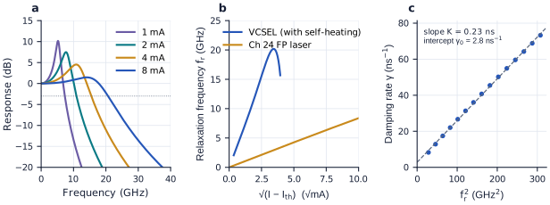
The relaxation-oscillation frequency \(f_r\) is set by the differential gain \(a = \mathrm{d}g/\mathrm{d}N\), the photon density \(S\) and the photon lifetime. Because \(S\) grows linearly with \(I - I_\mathrm{th}\), \(f_r\) grows as \(\sqrt{I - I_\mathrm{th}}\). Physically, carriers and photons pass energy back and forth: extra carriers raise the gain, which raises the photon density, which burns the carriers down again. The damping \(\gamma\) grows as \(f_r^2\) through the K-factor, \(K = 4\pi^2(\tau_p + \varepsilon/(v_ga))\), which includes gain compression. The damping eventually flattens and lowers the response, capping the bandwidth near \(2\pi\sqrt{2}/K\).
With \(a = 4.6\times10^{-16}\) cm² at threshold (\(g_0/N_\mathrm{th}\)), \(\tau_p = 2.76\) ps and \(\varepsilon = 2\times10^{-17}\) cm³, the laser has \(f_r = 4.7\) GHz and a 3 dB bandwidth of 7.2 GHz at 50 mA. At 120 mA these are 8.4 and 12.6 GHz. Its K-factor is 314 ps, so no bias can take its bandwidth beyond about 28 GHz. Lasers built for direct modulation at 25–50 Gb/s use quantum wells with several times this differential gain, short cavities and small active volumes.
A VCSEL reaches such speeds at a few milliamperes (Figure 25.1). Substituting the steady-state photon density into \(f_r\) gives \(f_r \approx D\sqrt{I - I_\mathrm{th}}\), with the D-factor \(D = \frac{1}{2\pi}\sqrt{\Gamma v_g a\eta_i/(qV)}\): the smaller the active volume, the more photons per unit volume each milliampere buys. The VCSEL of Section 24.8, with 59 times less volume, has \(D = 6.1\) GHz/√mA against 0.85 GHz/√mA for the Chapter 24 laser. At 8 mA it has \(f_r = 17.5\) GHz and a 3 dB bandwidth of 20.7 GHz, including the electrical parasitics of Section 25.8 (25.1 GHz without them). Two effects end the climb. The damping grows as \(Kf_r^2\), with \(K = 0.23\) ns for this VCSEL, which caps the bandwidth near 38 GHz. Self-heating acts first: above 12 mA the warm active region loses gain, and \(f_r\) peaks at 20.2 GHz and falls. At low bias the response is weakly damped: at 1 mA it peaks 10.2 dB high at 5.2 GHz, which matters when the zero level of a modulated laser is set low (Section 25.7).
figsrc/ch2x_lasers.py.25.2Chirp and the α-factor
In a semiconductor, a change of carrier density changes the refractive index as well as the gain (Chapter 19 describes the same physics in silicon). The ratio of the two is the linewidth-enhancement factor,
\[\alpha = -\frac{4\pi}{\lambda}\,\frac{\mathrm{d}n/\mathrm{d}N}{\mathrm{d}g/\mathrm{d}N},\]typically 2–6 for quantum-well lasers. Under direct modulation the frequency then follows the power, \(\Delta\nu(t) = \frac{\alpha}{4\pi}\left(\frac{\mathrm{d}\ln P}{\mathrm{d}t} + \kappa P\right)\): a transient term at the edges of each bit and an adiabatic term that follows the power level. This chirp broadens the spectrum. Over dispersive fibre it smears the pulses, which is why directly modulated lasers are confined to short reaches or to the dispersion-free 1310 nm window, and longer links use external modulators (Chapter 20).
25.3Relative intensity noise
Spontaneous emission adds photons with random phases, and the discreteness of carriers and photons adds shot noise. The result is relative intensity noise, the power spectral density of the intensity fluctuations normalised to the mean power squared, in dB/Hz. Because the noise sources are filtered by the same laser dynamics, RIN peaks at the relaxation-oscillation frequency and falls at higher power, roughly as \(1/P^3\) below the peak, until it meets the shot-noise floor \(2h\nu/P\). Good DFB lasers reach below −150 dB/Hz. Intensity-modulated links need RIN well below the receiver’s other noise (Chapter 21); analogue and coherent links are more demanding still.
25.4Phase noise and linewidth
Each spontaneous photon that joins the lasing mode adds a small random phase, and the phase random-walks: the laser line has a finite width. Schawlow and Townes derived it for lasers in general; Henry showed that in semiconductors the coupling of gain and index enhances it by \(1 + \alpha^2\) [44]:
with \(\Gamma g_\mathrm{th} = \alpha_i + \alpha_m\) the modal gain at threshold, \(P_0\) the power from one facet of a symmetric laser and \(n_{sp}\) the population-inversion factor. The linewidth falls as \(1/P_0\), since each spontaneous photon matters less among more photons. It also falls with lower cavity loss, which means longer photon lifetimes.
Try it. Raise the bias, shorten the cavity and change α. The plots show the modulation response, the RIN and the linewidth against power.
For the Chapter 24 laser at 6.5 mW per facet, \(n_{sp} = 1.8\) and \(\alpha = 4\), the linewidth is 2.1 MHz. Without the α-factor it would be 0.12 MHz, seventeen times narrower. Megahertz linewidths are fine for intensity-modulated links. Coherent links with high-order formats need about 100 kHz or less, FMCW LiDAR needs coherence over its ranging distance (Chapter 34), and atomic and quantum applications need hertz.
25.5Optical feedback
Light reflected back into a laser, from a fibre connector, a grating coupler or a chip facet, interferes with the lasing field. Depending on its strength and delay, it can narrow the line slightly, cause mode hopping, or drive the laser into coherence collapse, where the linewidth explodes to gigahertz and the RIN rises by tens of decibels. Collapse can begin at feedback levels of about −40 to −30 dB for typical lasers. Fibre-coupled lasers use optical isolators, which pass light one way only through the Faraday effect in magnetic garnets; on silicon there is no practical integrated isolator yet. Lasers on chip must therefore tolerate their own reflections: low-reflection couplers (Chapter 15), angled facets, quantum-dot gain with its small α-factor, or a deliberately strong, controlled feedback that dominates the stray reflections.
25.6Narrowing the linewidth
The linewidth formula suggests the cures: more photons in the cavity, and lower loss per round trip. An external cavity, with the gain chip coupled to a long, low-loss silicon or silicon-nitride waveguide circuit, stores the light for longer. To first order, the linewidth falls with the square of the ratio of the total optical length to the gain section’s. Detuning the lasing mode onto the slope of a ring filter adds a further reduction. With high-Q silicon-nitride rings, self-injection locking, where the ring’s backscatter locks the laser to the ring’s resonance, has reached sub-kilohertz fundamental linewidths in chip-scale lasers [50]. These designs are the subject of the next chapter.
25.7Driving a laser: bias, modulation and extinction ratio
Above threshold the output follows the current along a straight line, so a directly modulated laser is driven with current. In a current-mode driver, a differential pair steers a modulation current \(I_\mathrm{mod}\) either through the laser or into a dummy load, and a separate source supplies the bias [79]. Steering the current, rather than switching it on and off, keeps the supply current constant, so the driver does not shake its own supply. If the modulation current reaches the laser directly (DC coupling), the bias is the zero level: \(I_0 = I_\mathrm{bias}\) and \(I_1 = I_\mathrm{bias} + I_\mathrm{mod}\). If it passes through a capacitor (AC coupling), the bias is the average and the levels are \(I_\mathrm{bias} \pm I_\mathrm{mod}/2\).
A real transmitter never switches the light fully off. The ratio of the two power levels is the extinction ratio, and their difference, the optical modulation amplitude (OMA), is what the receiver actually sees [78]:
A receiver whose sensitivity is quoted as an average power \(\bar P\) needs more of it when the extinction ratio is finite: 1.1 dB more at an ER of 9 dB, 2.2 dB at 6 dB and 4.8 dB at 3 dB. Many recent link specifications therefore quote the transmitter’s OMA and the receiver’s OMA sensitivity instead, which removes this bookkeeping [78].
Why not set the zero level at threshold and take a large extinction ratio? Figure 25.2 shows what goes wrong, for the VCSEL of Section 24.8 driven at 25 Gb/s with its one level at 8 mA, simulated from the rate equations:
- Turn-on delay. Below threshold, every 1 must first refill the carriers (Chapter 24), which takes \(\tau_d = \tau_n\ln[(I_1 - I_0)/(I_1 - I_\mathrm{th})]\) [79]. With \(\tau_n = 2.4\) ns this is 52 ps from \(I_0 = 0\), longer than the 40 ps bit, and 22 ps from 0.1 mA. The delay depends on how long the laser was dark before, so it turns into data-dependent jitter.
- Ringing. Just above threshold the relaxation frequency is low and the damping weak (Figure 25.1a), so each rising edge overshoots and rings for several bits.
- Chirp. The transient chirp \((\alpha/4\pi)\,\mathrm{d}\ln P/\mathrm{d}t\) is largest when \(P_0\) is small. With \(\alpha = 4\), the peak-to-peak frequency swing is 167 GHz at \(I_0 = 0\), 69 GHz at 2 mA and 24 GHz at 5 mA.
Raising the zero level cures all three, but lowers the extinction ratio and the OMA. In the simulation the eye is closed for \(I_0 \le 0.25\) mA, opens at 0.5 mA, and is largest, 2.0–2.3 mW, for \(I_0\) between 0.75 and 2.25 mA (an ER of 11 to 6 dB). Above that it shrinks with the OMA, to 1.3 mW at 5 mA, where the ER is only 2.1 dB. Driving far above threshold buys speed with power [79].
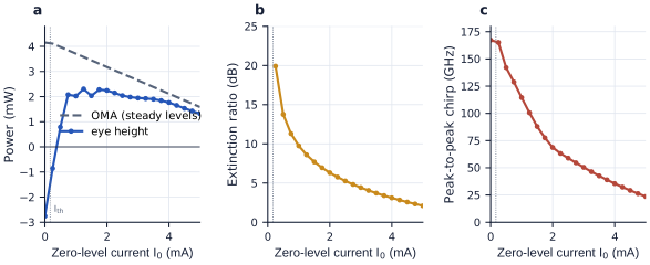
figsrc/ch2x_lasers.py.Choose \(I_0 = 2\) mA and \(I_1 = 8\) mA: a DC-coupled driver supplies a 2 mA bias and switches 6 mA, an AC-coupled one a 5 mA bias and ±3 mA. The junction settles at 45 °C, and the levels are \(P_0 = 0.97\) mW and \(P_1 = 4.15\) mW: an ER of 4.28 (6.3 dB), an OMA of 3.18 mW and an average of 2.56 mW. A receiver specified by average power pays 2.1 dB for the finite ER. The eye is 2.25 mW high, 71 % of the OMA; the rest is closed by ringing and the finite bandwidth. The laser draws 10.5 mW, and its chirp of 69 GHz peak-to-peak (0.17 nm at 850 nm) is harmless over a hundred metres of multimode fibre, whose own modal dispersion dominates.
25.8The laser as a circuit, and equalisation
Laser and driver are designed together, so the laser must exist as a circuit element. A compact model has three parts [79, 94]. The electrical part is the device’s impedance: the bond-pad capacitance, the series resistance of the doped mirrors or cladding, and the junction’s capacitance and nonlinear diode, with its turn-on voltage. The optical part is the rate equations, or their small-signal form: a second-order low-pass with \(f_r = D\sqrt{I - I_\mathrm{th}}\) and damping \(\gamma = Kf_r^2 + \gamma_0\). A thermal part, a thermal resistance and capacitance driven by the dissipated power, sets the temperature on which the threshold, gain and leakage depend. Written in Verilog-A, such a model runs in the circuit simulator beside the driver’s transistors.
Its parameters come from four measurements: the L–I curve gives the threshold and slope efficiency; the V–I curve the turn-on voltage and series resistance; the electrical reflection \(S_{11}\) over frequency the parasitic network; and the modulation response \(S_{21}\) at several biases gives \(D\), \(K\) and \(\gamma_0\). Plotting the fitted damping against \(f_r^2\) gives a straight line, whose slope is \(K\) and whose intercept is \(\gamma_0\): 0.23 ns and 2.8 ns⁻¹ for the example VCSEL (Figure 25.1c). The simulations in this chapter use such a model: a 120 fF pad, 70 Ω of mirror resistance and a 250 fF junction with a diode (ideality 2) in front of the rate equations of Section 24.8, at the junction temperature set by the average dissipated power.
The laser with its parasitics is a low-pass channel that rings, and a channel can be equalised at the transmitter, as electrical serial links do [84]. A feed-forward equaliser (FFE, or FIR filter) in the driver sets each bit’s current from the bit and its neighbours,
\[I[n] = \frac{I_0 + I_1}{2} + \frac{I_1 - I_0}{2}\sum_k c_k\,d[n - k], \qquad d = \pm 1,\]with one differential pair per tap, its tail current setting the weight \(c_k\), all summed at the laser [79]. Choosing \(\sum_k c_k = 1\) leaves the steady 0 and 1 levels, and hence the extinction ratio and average power, unchanged; the taps reshape only the transitions. Two constraints remain: the total current must stay above threshold, or the turn-on delay returns, and below the current the laser tolerates.
Figure 25.3 shows why this is worth doing. At 5 mA average current (levels of 2 and 8 mA) the 25 Gb/s eye is open, 71 % of the OMA. Lowering the average to 3 mA (1 and 5 mA) cools the junction from 45 to 35 °C, which lengthens the laser’s life, but leaves the zero level ringing near 5 GHz, and the eye shrinks to 29 %. A four-tap FIR, \(c = (-0.1, 0.9, 0.1, 0.1)\) for the bit before, the bit itself and the two after, reopens it to 52 %, with the current staying between 0.6 and 5.4 mA. These taps, the best of a grid search on this model, are not the classic pre-emphasis that boosts every transition. They push the current slightly the wrong way one bit before each transition, then step towards the new level over the next two bits, which cuts the drive by 18 % at 6.25 GHz, near the zero level’s relaxation frequency, while passing DC and the 12.5 GHz Nyquist frequency unchanged. The equaliser inverts whatever the laser does. When the laser and its parasitics are too slow rather than ringing, classic pre-emphasis wins: at 40 Gb/s with the 2 and 8 mA levels, the same search returns a negative first post-cursor, \((-0.1, 1.1, -0.1, 0.1)\), and lifts the eye from 17 % to 33 % of the OMA.
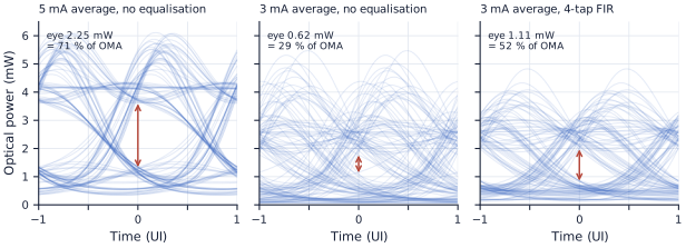
figsrc/ch2x_lasers.py.A linear FIR treats rising and falling edges alike, but a laser does not: it rises from the zero level, where it is slow and weakly damped, and falls from the one level, where it is fast. Drivers for VCSELs and directly modulated ring lasers therefore give the edges separate taps, one acting only after rising edges and one only after falling edges, each of either sign [94, 79]. In the 3 mA case above, a single tap that softens falling edges alone, holding the first 0 after each 1 at 30 % of the swing above the zero level, lifts the eye from 29 % to 46 % of the OMA. For four-level PAM4 signals the levels themselves sit at different biases, and drivers use level-dependent taps or look-up tables. A different, optical cure is injection locking: light injected from a master laser locks the laser’s frequency and raises its resonance several times above \(f_r\), extending the bandwidth of lasers that are slow on their own [94].
25.9Output stages and temperature control
The output stage. The driver’s output transistors must stay saturated above the laser’s forward voltage, 2.2 V for the VCSEL at 8 mA, so laser drivers in CMOS use thick-oxide transistors on a higher supply than the logic, or a separate driver chip [79]. A laser at the end of a bond wire or a short line is a poor impedance match, so the driver usually terminates the line with an on-chip resistor that absorbs reflections. That resistor also takes current: a 50 Ω termination beside a laser with 80 Ω of differential resistance passes only 38 % of the modulation current to the laser, so 6 mA of modulation needs 15.6 mA from the driver. Active back-termination, which drives the far end of the termination resistor with a replica of the output so that no signal current flows in it, and voltage-mode drivers recover most of that waste [79, 95]. Inductive peaking and a continuous-time equaliser in the output stage extend the bandwidth further.
Temperature. As a laser warms, its threshold rises (Chapter 24) and its slope efficiency falls. A driver holds the average power with automatic power control (APC): a monitor photodiode, on an edge emitter’s rear facet or a tap, feeds a slow loop that sets the bias. That fixes \(\bar P\) but not the extinction ratio, so the modulation current must also follow the slope efficiency, either from a look-up table indexed by a temperature sensor or by a second loop that measures the modulation amplitude in the monitor photocurrent.
The Chapter 24 laser. For \(P_0 = 1\) mW and \(P_1 = 5\) mW per facet (ER 7 dB) at 25 °C, the currents are 24.0 and 43.1 mA (\(I_\mathrm{mod}\) = 19.1 mA). At 85 °C the threshold is 52.2 mA, so the same powers need 57.0 and 76.1 mA. Without APC, both of the old currents would sit below the hot threshold and the laser would go dark. In this model the slope efficiency does not change with temperature, so APC alone, moving the bias by 33 mA, restores both levels.
The VCSEL. For \(P_0 = 0.8\) mW and \(P_1 = 3.2\) mW (an average of 2 mW, ER 6 dB), the currents are 1.68 and 6.20 mA at 25 °C ambient, with the junction at 39 °C. At 85 °C ambient the junction reaches 103 °C; the threshold has moved only from 0.17 to 0.26 mA, but leakage has cut the slope from 0.53 to 0.46 W/A. The currents become 2.00 and 7.21 mA: the modulation current must grow 15 %, from 4.52 to 5.21 mA. With APC alone, holding 2 mW average but leaving \(I_\mathrm{mod}\) at its 25 °C value, the extinction ratio drops from 6.0 to 5.0 dB.
Modulator drivers. External modulators need voltage rather than current: the travelling-wave electrode of a Mach–Zehnder modulator is a terminated line that needs a swing of volts, and a ring modulator is a small capacitor (Chapter 20). Their drivers are voltage-mode circuits, and the laser behind them needs only the bias half of a laser driver.
The reference link does not modulate its lasers directly: four continuous-wave lasers at 1550 nm feed ring modulators (Chapter 20), so chirp and relaxation oscillations do not limit it. The requirements on its lasers are RIN below about −140 dB/Hz, and tolerance of the grating couplers’ back-reflections (Chapter 15). Each needs only a constant current under automatic power control (Section 25.9).
Reading
- [4] Larry A. Coldren, Scott W. Corzine and Milan L. Mašanović. Diode Lasers and Photonic Integrated Circuits, 2nd edition. Wiley, 2012.
- [44] Charles H. Henry. “Theory of the linewidth of semiconductor lasers.” IEEE Journal of Quantum Electronics, 18(2):259–264, 1982.
- [50] Chao Xiang et al. “High-performance lasers for fully integrated silicon nitride photonics.” Nature Communications, 12:6650, 2021. Open access.
- [78] Sam Palermo. “Lecture 7: Transmitter Analysis.” ECEN 721: Optical Interconnects Circuits and Systems, Texas A&M University, Spring 2026. https://people.engr.tamu.edu/spalermo/ecen689_oi/lecture7_ee721_tx_analysis.pdf
- [79] Sam Palermo. “Lecture 8: VCSEL TXs.” ECEN 721: Optical Interconnects Circuits and Systems, Texas A&M University, Spring 2026. https://people.engr.tamu.edu/spalermo/ecen689_oi/lecture8_ee721_vcsel_tx.pdf
- [94] Sam Palermo. “Lecture 12: Laser Sources.” ECEN 721: Optical Interconnects Circuits and Systems, Texas A&M University, Spring 2026. https://people.engr.tamu.edu/spalermo/ecen689_oi/lecture12_ee721_laser_sources.pdf
- [84] Sam Palermo. “Lecture 7: Equalization Introduction & TX FIR Eq.” ECEN 720: High-Speed Links Circuits and Systems, Texas A&M University, Spring 2025. https://people.engr.tamu.edu/spalermo/ecen689/lecture7_ee720_eq_intro_txeq.pdf
- [95] Sam Palermo. “Lecture 5: Termination, TX Driver, & Multiplexer Circuits.” ECEN 720: High-Speed Links Circuits and Systems, Texas A&M University, Spring 2025. https://people.engr.tamu.edu/spalermo/ecen689/lecture5_ee720_termination_txdriver.pdf
- Direct modulation responds like a damped oscillator: \(f_r \propto \sqrt{I - I_\mathrm{th}}\), and damping \(Kf_r^2\) caps the bandwidth near \(2\pi\sqrt{2}/K\) (28 GHz for the Chapter 24 laser).
- The α-factor couples gain and index: it causes chirp and broadens the linewidth by \(1 + \alpha^2\).
- RIN peaks at \(f_r\) and falls with power towards the shot-noise floor.
- Linewidth \(\propto (1 + \alpha^2)/P\): about 2 MHz for the example laser at 6.5 mW.
- Feedback above about −40 dB can destabilise a laser; long low-loss external cavities and self-injection locking narrow the line by orders of magnitude.
- \(f_r = D\sqrt{I - I_\mathrm{th}}\) with \(D \propto 1/\sqrt{V}\): 6.1 GHz/√mA for the example VCSEL against 0.85 for the edge emitter. A compact model (parasitics, rate equations or \(D\), \(K\), \(\gamma_0\), a thermal node) lets laser and driver be simulated together.
- ER = \(P_1/P_0\) and OMA = \(P_1 - P_0\); an average-power receiver pays \((\mathrm{ER}+1)/(\mathrm{ER}-1)\), 2.2 dB at 6 dB. A zero level near threshold brings turn-on delay (52 ps from 0 mA), ringing and chirp (167 GHz peak-to-peak); a high one wastes ER. The 25 Gb/s VCSEL eye is best for zero levels of 0.75–2.25 mA.
- A FIR equaliser in the driver must invert the laser’s own response: at 3 mA average it reopened the VCSEL’s eye from 29 % to 52 % of the OMA. Rising and falling edges need different taps.
- APC tracks the threshold with the bias; the modulation current must also track the slope efficiency (+15 % for the VCSEL from 25 to 85 °C), or the extinction ratio falls.