Chapter 3Gaussian Beams and Optical Fibres
The beam that leaves a laser and the mode that travels down a fibre are both, to a very good approximation, Gaussian.
- derive the paraxial wave equation and its Gaussian-beam solution;
- compute a beam’s radius, wavefront curvature, Rayleigh range, divergence and Gouy phase;
- propagate a beam through lenses with the complex q-parameter and ABCD matrices;
- describe standard single-mode fibre: V-number, cut-off, mode-field diameter, loss and dispersion bands;
- compute the coupling efficiency between two modes, including size mismatch, offset and tilt.
How much light gets from one Gaussian mode into another, and how precisely must the two be aligned?
3.1The paraxial wave equation
A laser beam is not a plane wave: it has a finite width, and so it must spread. To describe it, write the field as a fast carrier times a slowly varying envelope, \(E = A(x,y,z)\,e^{-jkz}\) with \(k = nk_0\), and substitute into the Helmholtz equation of Chapter 2:
\[\nabla_T^2 A + \frac{\partial^2A}{\partial z^2} - 2jk\frac{\partial A}{\partial z} = 0.\]If the envelope changes little over a wavelength along \(z\), \(\lvert \partial^2A/\partial z^2\rvert \ll \lvert 2k\,\partial A/\partial z\rvert\), and the middle term can be dropped. What remains is the paraxial wave equation,
\[\nabla_T^2 A = 2jk\frac{\partial A}{\partial z},\]which has the same form as the diffusion equation and the Schrödinger equation. It holds for beams whose rays make small angles with the axis, which in practice means divergence half-angles below about 20–30°.
3.2The Gaussian beam
The lowest-order solution of the paraxial equation is the Gaussian beam:
Here \(r\) is the distance from the axis, \(w(z)\) the beam radius (where the intensity has fallen to \(1/e^2\) of its peak; twice it is the mode-field diameter, MFD), \(w_0\) the radius at the waist, \(R(z)\) the radius of curvature of the wavefronts, and \(\zeta(z)\) the Gouy phase, an extra phase of π/2 that the beam slips through on each side of its focus.
The Rayleigh range \(z_R\) is the distance over which the beam stays nearly collimated: there its area has doubled. Far from the waist the beam spreads as a cone with half-angle
\[\theta_0 \approx \frac{\lambda_0}{\pi n w_0}.\]A small spot diverges fast and a large one slowly, a direct consequence of diffraction. The fraction of the power inside a radius \(w\) is \(1 - e^{-2} = 86.5\ \%\). Real beams are not perfect Gaussians; the factor \(M^2 \geq 1\) by which a beam diverges faster than a Gaussian of the same waist measures how far from ideal it is.
The output of a semiconductor laser or a silicon edge coupler might have \(w_0 = 1.5\) µm. At 1550 nm in air its Rayleigh range is \(\pi(1.5)^2/1.55 = 4.6\) µm and it diverges at \(\theta_0 = 1.55/(\pi\times1.5) = 0.33\) rad, or 19°. The mode of a standard single-mode fibre has \(w_0 \approx 5.2\) µm: \(z_R = 55\) µm and \(\theta_0 = 5.4°\). Butt-coupling the small spot straight into the fibre therefore needs a gap well below 5 µm, and even then the spot sizes do not match (Section 3.5). A lens, or a mode converter on the chip, is needed.
3.3Beam transformation with q and ABCD
The beam radius and the wavefront curvature combine into one complex number, the q-parameter:
\[\frac{1}{q(z)} = \frac{1}{R(z)} - j\frac{\lambda_0}{\pi n w(z)^2}, \qquad q(z) = z + jz_R \ \ \text{(measured from the waist)}.\]Its power is that any paraxial optical system described by a ray-transfer matrix \(\begin{pmatrix}A & B\\ C & D\end{pmatrix}\) transforms it by one rule [41]:
Chaining matrices for a sequence of elements and applying the law once gives the beam anywhere. For a beam with waist \(w_0\) a distance \(d_1\) before a thin lens, the lens forms a new waist \(w_0' = M w_0\) at a distance \(d_2\) behind it, with
\[M = \frac{f}{\sqrt{(d_1 - f)^2 + z_R^2}}, \qquad d_2 = f + \frac{(d_1 - f)f^2}{(d_1 - f)^2 + z_R^2}.\]When \(z_R \ll \lvert d_1 - f\rvert\) these reduce to the familiar ray-optics magnification and imaging condition.
Image the 1.5 µm spot of Example 3.1 (\(z_R = 4.6\) µm) with a lens of focal length \(f = 100\) µm placed \(d_1 = 130\) µm away:
\[M = \frac{100}{\sqrt{30^2 + 4.6^2}} = 3.30, \qquad w_0' = 4.94\ \mu\mathrm{m}, \qquad d_2 = 100 + \frac{30\times100^2}{30^2 + 4.6^2} = 426\ \mu\mathrm{m}.\]A fibre with \(w = 5.2\) µm placed 426 µm behind the lens collects 99.7 % of the light (Section 3.5). Micro-lenses and ball lenses in laser packages do exactly this.
Try it. Focus the source with the lens, move the fibre, and watch the coupling and its tolerance.
3.4Optical fibres
A step-index fibre has a core of radius \(a\) and index \(n_1\) inside a cladding of index \(n_2\), slightly lower. Its guiding strength is summed up by the numerical aperture and the V-number:
with \(\Delta = (n_1 - n_2)/n_1\). Because \(\Delta\) is small (0.3–0.4 % in standard fibre), the modes are almost linearly polarised and are labelled LP\(_{lm}\) [63]. Solving the wave equation in the core (Bessel functions \(J_l\)) and the cladding (modified Bessel functions \(K_l\)) and matching them at \(r = a\) gives the characteristic equation
\[u\,\frac{J_{l-1}(u)}{J_l(u)} = -w\,\frac{K_{l-1}(w)}{K_l(w)}, \qquad u^2 + w^2 = V^2,\]where \(u\) and \(w\) are the transverse wavenumbers in the core and cladding scaled by \(a\). The fundamental mode LP\(_{01}\) is always guided; the next, LP\(_{11}\), appears at \(V = 2.405\), the first zero of \(J_0\). The cut-off wavelength \(\lambda_c = 2\pi a\,\mathrm{NA}/2.405\) is the shortest wavelength at which the fibre is single-mode.
Near cut-off the LP\(_{01}\) field is close to a Gaussian, and its radius is well approximated by Marcuse’s formula [62]:
\[\frac{w}{a} \approx 0.65 + \frac{1.619}{V^{3/2}} + \frac{2.879}{V^6}.\]Take a core radius of 4.1 µm and \(\Delta = 0.36\ \%\), close to standard (G.652) fibre [57]. With \(n_2 = 1.444\), \(n_1 = 1.449\) and NA = 0.123. The cut-off is \(\lambda_c = 2\pi\times4.1\times0.123/2.405 = 1.32\) µm, so the fibre is single-mode through the O band and beyond. At 1550 nm, \(V = 2.04\) and Marcuse gives \(w = 5.10\) µm, an MFD of 10.2 µm; at 1310 nm, \(V = 2.42\) and MFD = 9.0 µm. Data sheets quote about 10.4 and 9.2 µm, measured rather than modelled.
Try it. Change the core radius, NA and wavelength, and see which LP modes are guided and how well LP01 matches a Gaussian.
Silica fibre is used in five telecom bands: O (1260–1360 nm), E (1360–1460), S (1460–1530), C (1530–1565) and L (1565–1625 nm). Loss is about 0.35 dB/km in the O band and about 0.2 dB/km in the C band, where it is lowest; the C and L bands are also where erbium-doped amplifiers work. Chromatic dispersion is close to zero near 1310 nm and about 17 ps/(nm·km) at 1550 nm (Chapter 2).
Three special fibres appear in photonic-chip work. Polarisation-maintaining (PM) fibres have stress rods that make them strongly birefringent, so light launched along one axis stays there; fibre arrays for testing grating couplers usually use them (Chapter 17). High-NA fibres have small cores and spots of about 3–4 µm, closer to on-chip modes. Lensed fibres have a shaped tip that focuses the mode to a spot of about 2–3 µm for edge coupling (Chapter 16).
3.5Mode overlap and coupling efficiency
When light in one mode \(E_1\) arrives at a plane where it must enter another mode \(E_2\), such as at a fibre facet or a waveguide junction, the fraction of power coupled is the overlap integral:
\[\eta = \frac{\left\lvert \iint E_1E_2^*\,\mathrm{d}A\right\rvert ^2}{\iint\lvert E_1\rvert ^2\,\mathrm{d}A\iint\lvert E_2\rvert ^2\,\mathrm{d}A}.\]The rest is reflected or radiated. For two circular Gaussian modes with radii \(w_1\) and \(w_2\), flat wavefronts and parallel axes, the integral has closed forms:
and two equal modes separated by an axial gap \(z\) couple \(\eta = 1/\left[1 + (z/2z_R)^2\right]\). Figure 3.1 plots the first two factors.
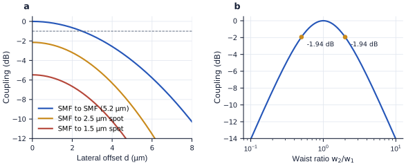
figsrc/part1_figs.py.Butt-coupling a standard fibre (\(w = 5.2\) µm) to a 1.5 µm on-chip spot gives \(\eta = (2\times5.2\times1.5/29.29)^2 = 0.28\), or −5.5 dB, before any misalignment; a 2.5 µm spot gives −2.2 dB. Between two standard fibres, the 1 dB tolerances are a lateral offset of \(d = \sqrt{0.115\times2\times5.2^2} = 2.5\) µm and a tilt of 2.6° in air. Because the tolerances scale with the spot size, an edge coupler that expands its mode to match the fibre is both more efficient and easier to align.
Coupling to fibre is a mode-matching problem. On-chip silicon modes are a few hundred nanometres across and fibre modes ten micrometres, a factor of about twenty-five in diameter: without help, almost all the light is lost. Every fibre coupler in Part IV is a way of building a large, Gaussian-like mode on the chip, by diffraction from a grating (Chapter 15) or by an inverse taper that lets the mode expand (Chapter 16), and the alignment tolerances of Chapter 17 follow from the same overlap integral.
3.6Gaussian beams in photonic chips
Gaussian beams turn up wherever light leaves a waveguide. A grating coupler radiates a beam about the size of a fibre mode, tilted by around 10° from the vertical; its profile is closer to an exponential than to a Gaussian unless the grating is apodised, which costs about 1 dB of overlap (Chapter 15). An edge coupler produces a spot of a few micrometres at the facet, matched to a lensed or high-NA fibre (Chapter 16). A semiconductor laser emits an elliptical, strongly diverging beam, often tens of degrees in one direction and less in the other, which micro-optics reshape for a fibre or for a silicon chip (Chapter 27). And 3D-printed micro-lenses and photonic wire bonds now let the beam be shaped right at the chip (Chapter 17).
Reading
- [41] Herwig Kogelnik and Tingye Li. “Laser beams and resonators.” Applied Optics, 5(10):1550–1567, 1966.
- [2] Bahaa E. A. Saleh and Malvin C. Teich. Fundamentals of Photonics, 3rd edition. Wiley, 2019.
- [5] Anthony E. Siegman. Lasers. University Science Books, 1986.
- [8] Allan W. Snyder and John D. Love. Optical Waveguide Theory. Chapman and Hall, 1983.
- [63] D. Gloge. “Weakly guiding fibers.” Applied Optics, 10(10):2252–2258, 1971.
- [62] Dietrich Marcuse. “Loss analysis of single-mode fiber splices.” Bell System Technical Journal, 56(5):703–718, 1977.
- A Gaussian beam is set by its waist: \(z_R = \pi w_0^2n/\lambda_0\) and \(\theta_0 = \lambda_0/(\pi nw_0)\). Small spots diverge fast.
- The q-parameter and ABCD matrices propagate a beam through lenses and gaps; a lens images a waist with magnification \(f/\sqrt{(d_1 - f)^2 + z_R^2}\).
- Standard single-mode fibre is single-mode for \(V < 2.405\) (cut-off about 1.3 µm) and has an MFD of about 10.4 µm at 1550 nm and 9.2 µm at 1310 nm.
- Coupling is a mode overlap. A waist mismatch of two costs 1.9 dB; a 5.2 µm to 1.5 µm mismatch costs 5.5 dB; between fibres the 1 dB tolerance is about 2.5 µm laterally and 2.6° in tilt.
- Fibre couplers exist to build a large, Gaussian-like mode on the chip.