Lab 3 · SimulateDirectional Coupler and MMI Design in Python
Write a finite-difference mode solver in a dozen lines, use it with the effective-index method to find the supermodes of a directional coupler and the self-imaging length of an MMI, and measure how far the results are from the full-vectorial numbers of Chapters 9 and 10.
- collapse the vertical direction of a silicon device with the effective-index method of Lab 1;
- write a finite-difference mode solver for any lateral index profile, and check it against the exact slab;
- find the supermodes of two coupled strips, the cross-over length and the 3 dB coupler length, against gap and wavelength;
- find the modes and the beat length of an MMI’s multimode section;
- propagate a field through the MMI by eigenmode expansion and find its 1 × 2 splitting length.
What you need
- Chapter 9 (Sections 9.2 to 9.4) and Chapter 10 (Sections 10.2 to 10.4); Lab 1 helps.
- Python 3.11 or newer with NumPy and Matplotlib:
pip install numpy matplotlib. - The script
lab03_couplers.py(also in the repository’slabs/folder). - About two hours, including the exercises.
Run it from a terminal in the folder where you saved it:
python lab03_couplers.py
It prints a checkpoint for each part below, with the value from the chapter beside it, and saves the figure lab03_couplers.png in a few seconds. Read each part, then the matching function in the script; change things and run it again. All lengths are in micrometres.
The usual tools for this job are an FDTD solver such as MEEP or an eigenmode-expansion (EME) solver. This lab does the same job with NumPy alone, so that it runs anywhere and hides nothing: an effective-index reduction to two dimensions, a mode solver for the lateral profile, and an eigenmode expansion along the device. Going further points to the full tools.
L3.1Collapse the vertical direction
Every device in this lab is a 220 nm silicon film, etched into shapes seen from above: two strips side by side, or one wide section. The effective-index method of Lab 1 (Section 6.2) turns each into a one-dimensional problem across the chip: the film’s vertical slab mode gives an index \(n_\mathrm{I}\) wherever there is silicon, and the oxide keeps its own index everywhere else. vertical_index returns \(n_\mathrm{I}\) from slab_modes, copied from Lab 1, with the Sellmeier indices of silicon and oxide (n_si, n_ox), the same ones the chapters’ femwell solutions use.
The lateral problem takes the other polarisation. A TE-like mode’s electric field is horizontal, normal to the side walls, so its lateral slab is solved as TM, exactly as in Lab 1. That choice matters in L3.4.
At 1550 nm, \(n_\mathrm{Si} = 3.4764\) and \(n_\mathrm{ox} = 1.4440\), and the film’s TE0 index is \(n_\mathrm{I} = 2.8482\) (Chapter 5: 2.848; Chapter 10 rounds it to \(n_r = 2.85\)). Every lateral profile below is 2.8482 in the silicon and 1.4440 around it.
L3.2A finite-difference mode solver
For a TM slab, the lateral field \(H(x) = H_y\) obeys
\[\frac{\mathrm{d}}{\mathrm{d}x}\left(\frac{1}{n^2}\frac{\mathrm{d}H}{\mathrm{d}x}\right) + k_0^2 H = \frac{\beta^2}{n^2} H.\]Sample \(H\) at nodes a step \(h\) apart and replace the derivatives with differences. With \(a = 1/n^2\),
\[\frac{a_{i+1/2}\,(H_{i+1} - H_i) - a_{i-1/2}\,(H_i - H_{i-1})}{h^2} + k_0^2 H_i = \beta^2 a_i H_i .\]Each equation links a node to its two neighbours only, so the matrix is tridiagonal, and \(\beta^2\) is its eigenvalue. Substituting \(H_i = n_i v_i\) makes it symmetric, so numpy.linalg.eigh returns every mode at once, sorted, with orthonormal fields. Two details make it accurate:
- the grid is cell-centred and every wall falls halfway between two nodes (
grid), so each node sits in one material; - at a wall, \(a_{i+1/2} = 2/(n_i^2 + n_{i+1}^2)\): the average that keeps \((1/n^2)\,\mathrm{d}H/\mathrm{d}x\), which is proportional to \(E_z\), continuous.
The heart of fd_modes:
a = 1 / eps
a_mid = 2 / (eps[:-1] + eps[1:])                         # 1/n^2 halfway between neighbouring nodes
a_left, a_right = np.r_[a[0], a_mid], np.r_[a_mid, a[-1]]  # the field is zero just outside the window
diag = n * (k0**2 - (a_left + a_right) / h**2) * n
off = n[:-1] * a_mid * n[1:] / h**2
beta2, v = np.linalg.eigh(np.diag(diag) + np.diag(off, 1) + np.diag(off, -1))
The fields come back normalised so that \(\sum\lvert H\rvert^2/n^2\,h = 1\). With this weight the modes are orthonormal, which the eigenmode expansion of L3.5 relies on. tm=False solves the simpler TE equation, \(\mathrm{d}^2E/\mathrm{d}x^2 + k_0^2n^2E = \beta^2E\), for comparison.
For one 500 nm strip the solver gives \(n_\mathrm{eff}\) = 2.49258, 2.49204 and 2.49190 with steps of 20, 10 and 5 nm, and the exact lateral slab (Lab 1’s bisection) gives 2.49186. The error falls fourfold each time the step halves: the method is second order. Lab 1 found 2.4914 with \(n_\mathrm{Si} = 3.476\); the Sellmeier value, 3.4764, adds 0.0004. femwell’s full-vectorial answer is 2.446 (Chapter 6), so the EIM is 0.046 too high, as in Lab 1. Solving the lateral problem as TE instead gives 2.630, further off still.
L3.3Supermodes and the directional coupler
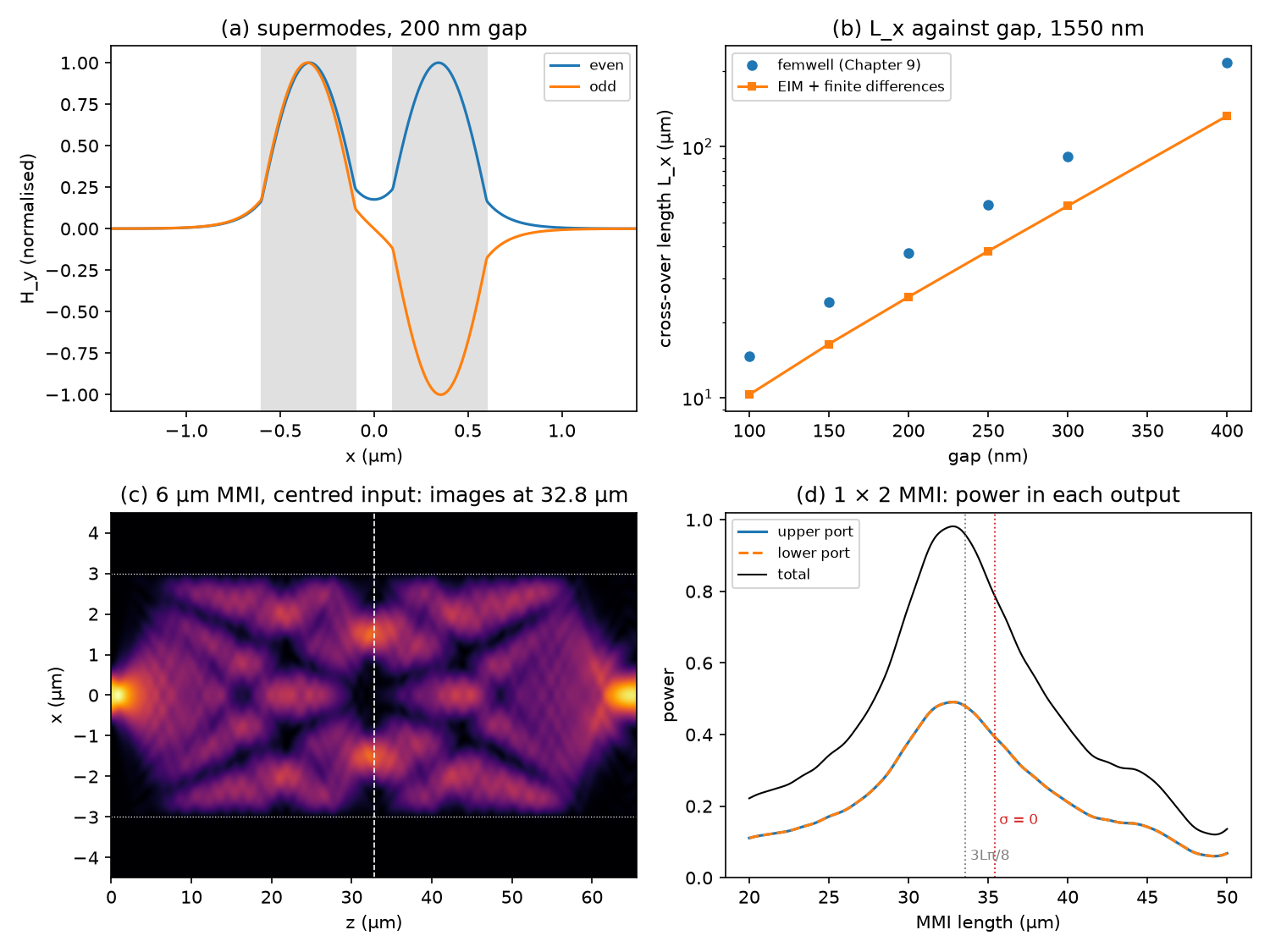
coupler(gap) builds the profile of two 500 nm strips and solves it. The two highest modes are the even and odd supermodes of Section 9.2, and crossover returns \(L_x = \lambda/(2(n_\mathrm{even} - n_\mathrm{odd}))\). The script carries femwell’s values for the same gaps (FEMWELL_LX, the data of Figure 9.1). A 3 dB coupler crosses \(\sin^2(\pi(L + L_b)/(2L_x))\) of the power (Section 9.3), so it needs \(L + L_b = L_x/2\), with \(L_b = 2.5\) µm contributed by the bends.
As a check on the supermode picture, expansion launches the mode of the left strip alone into the pair, expands it onto all of the pair’s guided modes, lets each travel with its own \(\beta\), and projects the result onto the mode of the right strip. The same function propagates through the MMI in L3.5.
At a 200 nm gap the EIM gives \(n_\mathrm{even} = 2.5092\) and \(n_\mathrm{odd} = 2.4785\), so \(L_x = 25.2\) µm, against femwell’s 2.4573, 2.4368 and 37.8 µm (Worked Example 9.1). From 100 to 400 nm gaps the EIM’s \(L_x\) is 0.70 down to 0.61 times femwell’s, and it grows 2.30 times per 100 nm against femwell’s 2.41 (Chapter 9: about 2.4). The 3 dB coupler needs \(L_x/2 = 12.61\) µm, a straight section of 10.1 µm with the bends (Chapter 9: 16.4 µm); the expansion crosses 50 % at 12.62 µm. At 1500 and 1600 nm, \(L_x\) = 30.9 and 20.8 µm (Chapter 9: 47 and 31 µm). A coupler set for 50 % at 1550 nm crosses 44.0 % at 1530 nm and 56.3 % at 1570 nm, a drift of 0.31 %/nm (Chapter 9: 43.5 %, 57 % and 0.35 %/nm).
The EIM gets the physics right: the exponential growth with the gap, the strong growth with wavelength, and so the drift of a 3 dB coupler, which depends only on how \(L_x\) changes with wavelength. But its coupling is 1.4–1.6 times too strong, and the error grows with the gap. The light that couples the two guides crosses the gap, exactly where the EIM’s central assumption, one vertical profile everywhere (Section 6.2), is worst: there is no silicon in the gap to hold that profile. Use the EIM to understand a coupler and to start a design; take the final length from a full-vectorial solver, as Chapter 9 does.
L3.4The MMI’s modes and its beat length
mmi_grid builds the 6 µm multimode section of Worked Example 10.1 on a 10 nm grid with 1.5 µm of oxide on each side, and fd_modes gives all its modes at once. The beat length is \(L_\pi = \pi/(\beta_0 - \beta_1) = \lambda/(2(n_0 - n_1))\) (Section 10.3), and the script compares it with the formula \(4n_rW_e^2/(3\lambda)\) for both values of \(\sigma\) in the effective width.
Which \(\sigma\)? The effective width adds the penetration of the field into the cladding at each wall, and that depends on the polarisation of the lateral slab: \(\sigma = 0\) for a field parallel to the walls (a TE slab), \(\sigma = 1\) for a field normal to them (TM), which shortens the penetration by \((n_c/n_r)^2 = 0.26\). A TE-like mode’s field is normal to the walls, so its lateral slab is TM (L3.1), and \(\sigma = 1\), as Section 10.3 says. The script also shows the field-parallel case, \(\sigma = 0\), for comparison.
The section guides 19 modes. The solver gives \(n_0 = 2.84531\) and \(n_1 = 2.83665\), so \(L_\pi = 89.5\) µm. The formula gives 89.7 µm with \(\sigma = 1\) and \(W_e = 6.052\) µm (Worked Example 10.1, with \(n_r = 2.85\): \(W_e = 6.052\) µm, \(L_\pi = 89.8\) µm). With \(\sigma = 0\) it would give 94.2 µm (\(W_e = 6.201\) µm), and solving the same section as TE gives 94.0 µm. Against the quadratic law \(\beta_0 - \beta_\nu = \nu(\nu + 2)\pi/(3L_\pi)\), the modes are off by 0.2 % for \(\nu = 2\), 2.3 % for \(\nu = 6\), 6.4 % for \(\nu = 10\) and 24 % for the last guided mode, \(\nu = 18\).
So the solver and the formula agree to 0.2 % once \(\sigma\) matches the polarisation, and each polarisation’s solver result sits next to its own formula: 89.5 against 89.7 µm, and 94.0 against 94.2 µm. Taking the wrong \(\sigma\) makes a TE section about 5 % too long. Does the full three-dimensional structure side with \(\sigma = 1\)? Exercise 2 checks it against femwell.
L3.5Self-imaging by eigenmode expansion
At the abrupt junction where the input meets the wide section, the input field is projected onto the section’s modes (Section 10.2). With the fields normalised as in L3.2,
\[c_\nu = \int \frac{H_\mathrm{in}\,\phi_\nu}{n^2}\,\mathrm{d}x,\]and at a distance \(z\) the field is \(\sum_\nu c_\nu\phi_\nu e^{-j\beta_\nu z}\). expansion does exactly this with the guided modes, and returns a function giving the power coupled into each output waveguide at any length: the overlap of the field with that waveguide’s mode. The input is the mode of a 1.5 µm access waveguide (the tapered access guides of Section 10.4), centred; the outputs are the same guides at \(\pm W_e/4\), with \(W_e = 6.044\) µm implied by the solver’s \(L_\pi\). golden_max finds the best length.
This is the simplest eigenmode expansion: one junction at each end, overlaps in the MMI’s own weighting, no reflections. Full EME solvers add the reflections and use vectorial modes.
The centred input puts 99.93 % of its power into guided modes and none into odd ones, so only even modes interfere (symmetric interference, Section 10.3). The two outputs collect 49.1 % each at 32.80 µm, an excess loss of 0.08 dB, while \(3L_\pi/8\) from the solver’s \(L_\pi\) is 33.57 µm (Chapter 10: 33.7 µm). Cut at 35.4 µm, the length \(\sigma = 0\) would give, this model’s outputs would collect 39.4 % each, a loss of 1.03 dB. The images peak at ±1.54 µm, against \(W_e/4 = 1.51\) µm (Chapter 10: ±1.51 µm).
The best length is 2.3 % shorter than \(3L_\pi/8\) because the higher modes run ahead of the quadratic law (Checkpoint D), so the images form a little early. This is why an MMI is finished with a simulation sweep around the formula’s length (Section 10.4), and why the polarisation in the formula matters: the 5 % difference in \(L_\pi\) between \(\sigma = 1\) and \(\sigma = 0\) is 1.7 µm of a 1 × 2 MMI, enough to cost 1 dB (Checkpoint E).
Exercises
- Gap tolerance. Change the 100 nm gap by ±10 nm with
crossover. How much does \(L_x\) change (Chapter 9: about 10 % for a 10 nm error)? And at 300 nm? - Which polarisation? For a strip 1 µm wide (
strips(x, (0.0,), 1.0, n_I, n_c)ongrid(2.0, H)), compare \(n_0 - n_1\) fromfd_modeswithtm=Trueandtm=Falseagainst femwell’s TE0 and TE1, 2.7461 and 2.4198 (the data of Figure 6.1). Which value of \(\sigma\) does that support? - Narrower and wider MMIs. Set
W_MMIto 4 and to 8 µm. How many modes are guided, and how do \(L_\pi\), the best 1 × 2 length and the excess loss change? - Bandwidth. Keep the 1550 nm length, 32.80 µm, and evaluate the 1 × 2 MMI at 1500, 1530, 1570 and 1600 nm (pass
lamtommi_grid,access_modeandexpansion). Compare it with the directional coupler of Checkpoint C. - A 2 × 2 MMI by paired interference. Move the input to \(x = W_e/6 = 1.01\) µm and the outputs to \(\pm W_e/6\). Where does it split 50/50, and how does that compare with \(L_\pi/2\) (Chapter 10: 45 µm)?
Answers
- \(L_x\) = 10.29 µm at 100 nm, 11.34 µm at 110 nm (+10.2 %) and 9.31 µm at 90 nm (−9.5 %). At 300 nm, +10 nm gives +8.6 %. In relative terms the sensitivity is set by how fast the evanescent tail decays, about 9–10 % per 10 nm at any gap, so in absolute terms it is largest for wide gaps and long couplers. femwell’s own points between 100 and 150 nm also give about 10 % per 10 nm (10.4 %), slightly more than the 9 % of the exponential fit over all the gaps.
- As TM: 2.7517 − 2.4470 = 0.305; as TE: 2.7744 − 2.5447 = 0.230; femwell: 0.326. At 0.8 µm: 0.473 and 0.336, against femwell’s 0.521. femwell’s spacing is 7 % (1 µm) and 10 % (0.8 µm) larger than the TM slab’s, but 42 % and 55 % larger than the TE slab’s, so \(\sigma = 1\) is the right choice for TE-like modes. The real side walls confine the mode even more tightly than the TM slab does, so the true \(L_\pi\) is, if anything, a little shorter than 89.5 µm.
- 4 µm: 13 guided modes, \(L_\pi\) = 40.0 µm (formula with \(\sigma = 1\): 40.2 µm), best 1 × 2 length 14.60 µm, loss 0.04 dB. 8 µm: 26 modes, 158.6 µm (158.8 µm), 57.85 µm, 0.14 dB. The length grows as \(W_e^2\): \((8.046/4.041)^2 = 3.96\), the ratio of the two lengths. The loss grows with width because the input, always 1.5 µm wide, excites modes up to the same transverse wavenumber, whose departure from the quadratic law is fixed, but it accumulates over a length that grows as \(W^2\). Both best lengths are about 2.7 % short of \(3L_\pi/8\).
- Excess loss 0.33, 0.11, 0.08 (1550 nm), 0.14 and 0.42 dB, and the split stays exactly 50/50 by symmetry. Across 1530–1570 nm the directional coupler’s split moves from 44.0 % to 56.3 %, while the MMI’s outputs stay equal and lose at most 0.14 dB: as \(L_\pi\) moves with wavelength, the images only blur. That is why Table 10.1 rates MMIs as broadband splitters.
- The two outputs collect 48.7 % each at 43.32 µm (97.4 % in all); the total peaks at 97.8 % at 43.70 µm, split 49.1/48.7. \(L_\pi/2\) is 44.76 µm from the solver and 45 µm in Worked Example 10.1 (\(\sigma = 0\) would give 47 µm). As for the 1 × 2, the image forms about 3 % before the formula’s length.
Going further
- femwell solves the full cross-section of the coupler and gives the numbers of Chapter 9 directly; Lab 2 uses it.
- meow is an open eigenmode-expansion solver: the same idea as L3.5, with vectorial modes, many sections and reflections, for tapers and S-bends too.
- MEEP simulates the coupler and the MMI in 2D or 3D FDTD, including the bends that this lab adds as a fixed 2.5 µm.
- The coupler and MMI demos of Chapters 9 and 10 run simplified versions of these models in your browser.