Lab 12 · Lasers and linksClose the Reference Link Budget
Add up the reference link block by block in a few lines of Python, derive the receiver’s sensitivity from its noise, simulate the crosstalk and dispersion penalties instead of assuming them, and trade the margin that is left for laser power.
- write the budget as a table of blocks, and compute the received power and the margin;
- compute the bit-error ratio from Q, and the sensitivity from the receiver’s noise and the extinction ratio;
- estimate the crosstalk of Lorentzian drop rings on the 400 GHz grid;
- push a 50 Gb/s NRZ eye through 2 km of fibre with FFTs and measure its dispersion penalty;
- add up the energy per bit and trade margin for laser power.
What you need
- Chapter 33 (Sections 33.2, 33.5 and 33.7), with Chapter 1 (Worked Example 1.1, Table 1.3), Chapter 21 (Section 21.6), Chapter 14 (Worked Example 14.1) and Chapter 2 (Worked Example 2.5).
- Python 3.11 or newer with NumPy and Matplotlib:
pip install numpy matplotlib. The error function is Python’s ownmath.erfc, so SciPy is not needed. - The script
lab12_link.py(also in the repository’slabs/folder). - About two hours, including the exercises.
Run it from a terminal in the folder where you saved it:
python lab12_link.py
It prints a checkpoint for each part below, with the value from the chapter beside it, and saves the figure lab12_link.png in a few seconds. Read each part, then the matching function in the script; change things and run it again. Powers are in dBm, losses and penalties in dB, and frequencies in GHz.
L12.1The budget as a table of blocks
Losses multiply, so in decibels a link budget is a subtraction (Section 1.5). The script keeps the reference link as a list of blocks, each with its loss for one wavelength, in the order the light meets them, and the penalties of Table 33.1 as a dictionary:
def link_blocks(km=FIBRE_KM, gc=3.0, fibre_db_per_km=FIBRE_DB_PER_KM):
    return [("ring modulator", 3.0),
            ("other rings, routing", 0.8),
            ("TX grating coupler", gc),
            (f"{km:g} km of fibre", fibre_db_per_km * km),
            ("two connectors", 1.0),
            ("RX grating coupler", gc),
            ("demux ring, routing", 1.5)]

PENALTIES = {"crosstalk": 0.5, "dispersion": 0.5, "drift and locking": 1.0, "ageing": 1.0}

def power_levels(p_laser, blocks):
    return p_laser - np.cumsum([loss for _, loss in blocks])
power_levels is the power after every block, a running subtraction from the laser’s +10 dBm; its last value is the received power. The margin is the key equation of Section 33.2, \(\text{margin} = P_\mathrm{launch} - \sum_i L_i - \sum_j \mathrm{penalty}_j - P_\mathrm{sens}\), with the sensitivity of −11.6 dBm that the next part derives. The extinction-ratio penalty is not in the dictionary: it is already inside that sensitivity. Writing the budget this way makes every “what if” a change of one argument: link_blocks(gc=4.0) for the measured couplers, link_blocks(km=10) for a longer fibre.
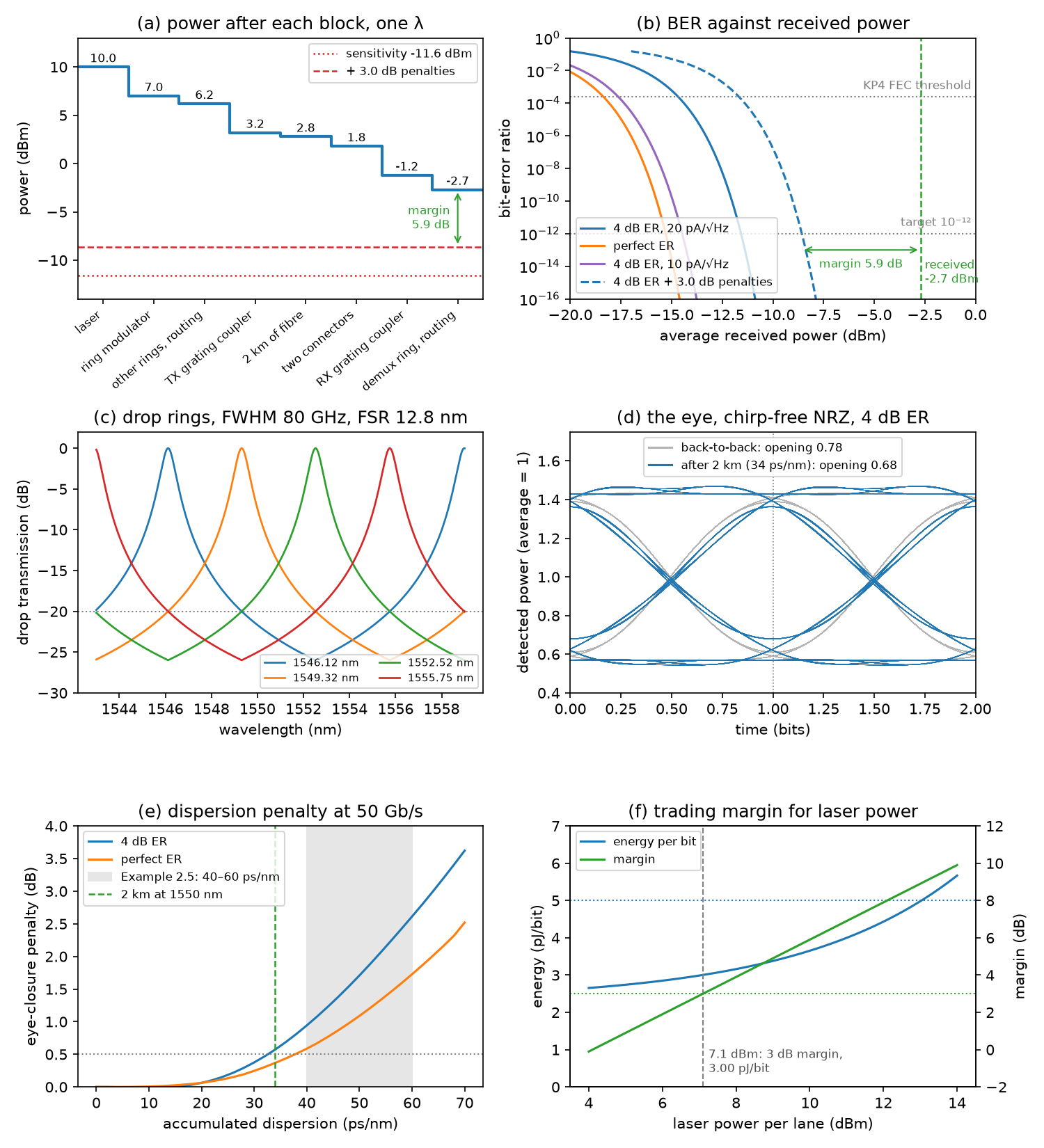
The losses add up to 12.7 dB, so the receiver gets −2.7 dBm (0.54 mW), 9.3 dB above the −12 dBm of Worked Example 1.1. After 3.0 dB of penalties the margin against −11.6 dBm is 5.9 dB. With the measured −4 dB grating couplers the receiver gets −4.7 dBm and the margin is 3.9 dB. All as in Table 33.1 and the text below it.
L12.2Bit-error ratio, Q and sensitivity
With Gaussian noise on the “0” and “1” levels, the bit-error ratio of NRZ depends only on the Q factor (Section 21.6): \(Q = (I_1 - I_0)/(\sigma_1 + \sigma_0)\) and \(\mathrm{BER} = \tfrac{1}{2}\,\mathrm{erfc}(Q/\sqrt{2})\). q_for_ber inverts it by bisection, since the BER falls steadily as Q rises. The receiver is the one of Worked Example 21.2: a germanium PIN of 0.9 A/W and a TIA with 20 pA/√Hz of input noise, over a noise bandwidth of 0.7 × 50 = 35 GHz. For an average power \(\bar P\) and a linear extinction ratio \(r\), the levels are \(P_1 = 2\bar P r/(r+1)\) and \(P_0 = 2\bar P/(r+1)\), so the optical modulation amplitude is \(2\bar P(r-1)/(r+1)\), only 0.86 times the average at 4 dB. q_factor adds each level’s shot noise and the dark current’s to the TIA’s noise:
def ber_from_q(q):
    return 0.5 * math.erfc(q / math.sqrt(2))

def q_factor(p_dbm, er_db=ER_DB, i_n=I_N, bit_rate=BIT_RATE, shot=True):
    bw = 0.7 * bit_rate
    p1, p0 = levels(p_dbm, er_db)
    i1, i0 = RESP * p1, RESP * p0
    var_th = i_n ** 2 * bw                          # the TIA: the same on both levels
    s1 = math.sqrt(var_th + (2 * Q_E * (i1 + I_DARK) * bw if shot else 0.0))
    s0 = math.sqrt(var_th + (2 * Q_E * (i0 + I_DARK) * bw if shot else 0.0))
    return (i1 - i0) / (s1 + s0)
sensitivity then finds, by bisection again, the lowest average power whose Q meets the target. With the TIA’s noise alone, the eye must be \(2Q\sigma\) tall, so the sensitivity follows in closed form; the shot noise of the “1” level adds a little. A finite extinction ratio wastes power on the “0”: against a perfect one it costs \(10\log_{10}[(r+1)/(r-1)]\) in a receiver dominated by its TIA, which is the extinction-ratio penalty of Section 33.2.
Q = 7.034 for 10⁻¹² and 3.49 for the KP4 threshold of 2.4 × 10⁻⁴ (Chapter 21: 7.03 and 3.49). The TIA’s noise is σ = 3.74 µA, so the eye needs \(I_1 - I_0 = 2Q\sigma = 52.6\) µA, an OMA of 58.5 µW, which at 4 dB of extinction (OMA/average = 0.861) is 67.9 µW, or −11.68 dBm (Worked Example 21.2: 68 µW, −11.7 dBm). Shot and dark-current noise move it to −11.57 dBm, the −11.6 dBm of Chapters 21 and 33. The 4 dB extinction ratio costs 3.66 dB: a perfect “0” gives −15.3 dBm, and 15 dB of extinction, the top of the Chapter 21 demo’s range, −15.0 dBm. KP4 FEC gives −14.7 dBm and a 10 pA/√Hz TIA −14.5 dBm (Chapter 21: −14.7 and −14.5 dBm). Against −11.57 dBm the link has 8.9 dB before penalties (Chapter 21: 8.9 dB).
L12.3Crosstalk from the drop rings
Each drop ring of the demultiplexer (Worked Example 14.1) has a Lorentzian response, \(T_\mathrm{drop} = 1/[1 + (2\Delta f/\Delta f_\mathrm{FWHM})^2]\), around each of its resonances, which repeat every FSR. The script works in frequency, because the ITU grid and a ring’s FSR are both even in frequency, not in wavelength. fwhm_for_rejection picks the width that rejects a channel 400 GHz away by 20 dB, and drop folds any detuning onto the nearest resonance. With an FSR of four channel spacings, 1600 GHz, every ring sees two neighbours 400 GHz away and the fourth channel 800 GHz away, half an FSR from both its resonances.
def drop(df, fwhm, fsr=FSR_GHZ):
    d = (np.asarray(df, dtype=float) + fsr / 2) % fsr - fsr / 2
    return 1 / (1 + (2 * d / fwhm) ** 2)

def crosstalk_penalty(x):
    return -10 * math.log10(1 - x)
The leaked channels are at other wavelengths, so they beat with the signal at 400 GHz and more, far outside the receiver’s bandwidth: the crosstalk is incoherent and simply adds power. At the worst pattern the neighbours’ “1”s land on the signal’s “0”s, and a fraction \(X\) of leaked power closes the eye by \(X\) of its height. A receiver dominated by its TIA needs that height back, so the penalty is \(-10\log_{10}(1 - X)\).
The channels are 1546.12, 1549.32, 1552.52 and 1555.75 nm (Table 1.3). −20 dB at 400 GHz needs a FWHM of 80.4 GHz (0.64 nm), a loaded Q of 2406, with an FSR of 1600 GHz (12.8 nm) (Worked Example 14.1: 0.64 nm, about 2400, 12.8 nm). Each neighbour leaks 1.00 % and the far channel 0.25 %: 2.25 % in all, a penalty of 0.10 dB (Chapter 33: about 2 %, roughly 0.1 dB, against an allowance of 0.5 dB). Filtering its own channel, the ring closes the eye by another 1.13 dB.
The last line runs the eye simulation of the next part with the ring in the signal’s path (the ring_fwhm argument). For the detected intensity, a Lorentzian of 80 GHz FWHM acts as a single-pole low-pass at 40 GHz, and in series with the transmitter and receiver it costs about a decibel (0.96 dB even with a perfect transmitter). Worked Example 14.1 calls this a small filtering penalty, and against 5.9 dB of margin it is; but Table 33.1 has no line for it. In practice it falls to the driver’s equalisation (Chapter 20), which the ring modulator’s 24 GHz optical bandwidth needs anyway.
L12.4Dispersion: a 50 Gb/s eye through 2 km
Worked Example 2.5 estimates the dispersion of 2 km of fibre with a rule of thumb; the script measures it. It builds a pseudo-random sequence of 511 bits (PRBS9, which contains every pattern of nine bits except all zeros), 32 samples per bit, and sends it through a transmitter with a Gaussian response 3 dB down at 35 GHz. A chirp-free modulator makes a real, positive field \(\sqrt{P(t)}\). The fibre multiplies the field’s spectrum by \(\exp(-i\beta_2L\omega^2/2)\), with \(\beta_2 L = -DL\lambda^2/(2\pi c) = -43\) ps² for \(DL = 34\) ps/nm. The photodiode squares the field, and the receiver is a fourth-order Bessel–Thomson filter 3 dB down at 37.5 GHz, the standard reference receiver for NRZ. The sequence repeats, so FFTs apply every filter exactly:
    drive = np.real(np.fft.ifft(np.fft.fft(np.repeat(bits, SPB).astype(float)) * gaussian_lowpass(f, f_tx)))
    p1, p0 = levels(30.0, er_db)                    # 30 dBm = 1 W: average power 1 (only ratios matter here)
    power = p0 + (p1 - p0) * drive
    field = np.sqrt(np.clip(power, 0, None))        # chirp-free: a real, positive field
    beta2L = -disp_ps_nm * 1e-3 * LAM ** 2 / (2 * np.pi * C)      # ps/nm = 1e-3 s/m; beta2L in s^2
    spectrum = np.fft.fft(field) * np.exp(-0.5j * beta2L * (2 * np.pi * f) ** 2)
    if ring_fwhm:
        spectrum = spectrum / (1 + 2j * f / (ring_fwhm * 1e9))
    field = np.fft.ifft(spectrum)
    detected = np.abs(field) ** 2                   # square-law photodiode
    return np.real(np.fft.ifft(np.fft.fft(detected) * bessel4_lowpass(f, f_rx)))
eye_opening cuts the waveform into bits and finds, at the best sampling time, the lowest “1” minus the highest “0”. The penalty is the ratio of the openings with and without the fibre, in decibels: the power a TIA-limited receiver needs to get its eye back. The transmitter and receiver alone already close the eye from 0.861 to 0.779 (0.43 dB); comparing against that back-to-back eye keeps the fibre’s share separate.
Why does the weakly modulated signal suffer more than a fully modulated one? At 4 dB of extinction most of the light is a steady carrier, and for a small modulation on a carrier, dispersion acts on the intensity as the filter \(\cos(\pi\lambda^2 DL f^2/c)\), which is already down to 0.86 at 25 GHz for 34 ps/nm.
34 ps/nm spread a 0.4 nm wide signal by 13.6 ps, most of a 20 ps bit (Worked Example 2.5: about 14 ps). The eye opening falls from 0.779 back-to-back to 0.683 after 2 km: a penalty of 0.57 dB, the “few tenths of a decibel” of Section 33.2, a little above its 0.5 dB allowance. With a perfect extinction ratio it is 0.37 dB, and without the transmitter’s filter 0.38 dB. The penalty reaches 1 dB at 41 ps/nm and 2 dB at 53 ps/nm, inside the 40–60 ps/nm tolerance of Worked Example 2.5. With this lab’s crosstalk (0.10 dB) and dispersion (0.57 dB) penalties in place of the allowances, the margin is 6.2 dB.
The two allowances together (1.0 dB) cover the two computed penalties (0.67 dB): the generous crosstalk allowance pays for the dispersion’s small overshoot. Drift, locking and ageing (2.0 dB) remain allowances, as in Table 33.1.
L12.5Energy per bit, and margin traded for laser power
The energy per bit of Section 33.5 adds the lasers’ wall-plug power, the heaters, the receivers, the drivers and the modulators, and divides by the total bit rate of 200 Gb/s. Eight rings at up to 20 mW each come from Worked Example 18.2; the TIA and driver energies are typical values.
def energy_per_bit(p_laser=P_LASER, wall_plug=WALL_PLUG, heater_mw=HEATER_MW):
    rate = N_LANES * BIT_RATE
    return {"lasers": N_LANES * 1e-3 * 10 ** (p_laser / 10) / wall_plug / rate * 1e12,
            "heaters": N_RINGS * heater_mw * 1e-3 / rate * 1e12,
            "TIAs": E_TIA, "drivers": E_DRIVER, "modulators": E_RING}
The laser term is the only one that scales with the margin. Any margin above the 3 dB target can be given back as laser power: cut each laser by the excess, and its wall-plug power falls by the same number of decibels.
1.33 + 0.80 + 1.00 + 0.50 + 0.02 = 3.65 pJ/bit (lasers, heaters, TIAs, drivers, modulators), as in Table 33.1. Each laser’s 10 mW of light draws 67 mW (Section 1.5), and the lasers are 36 % of the total. Cutting them by 2.9 dB to 7.1 dBm leaves exactly 3.0 dB of margin and saves 0.65 pJ/bit, for 3.00 pJ/bit in all (Chapter 33: 2.9 dB and 0.65 pJ/bit). Both targets are met: 5.9 dB of margin against 3 dB, and 3.65 pJ/bit against 5.
Exercises
- PAM4. Send the same 50 Gb/s as PAM4 at 25 GBd: four equally spaced levels between the same “1” and “0” powers (4 dB, same average), three eyes each a third of the OMA, and a noise bandwidth of 0.7 × 25 GHz. With Gray coding and equal eyes, \(\mathrm{BER} \approx \tfrac{3}{8}\,\mathrm{erfc}(Q/\sqrt{2})\), with \(Q\) for one eye. Write a PAM4 version of
q_factorand find the sensitivity and the margin with Table 33.1’s penalties. Why is the cost smaller than the 4.8 dB of Chapter 20? - The measured couplers. With
link_blocks(gc=4.0), what laser power restores 5.9 dB of margin, and what does it cost in energy? What is the lowest laser power that still keeps 3 dB? - Ten kilometres. Stretch the fibre to 10 km at 1550 nm (
link_blocks(km=10),dispersion_penalty(170)). Does the power budget close? Does the eye? How far can the link reach within the 0.5 dB dispersion allowance, and where does the eye close completely? Repeat in the O band, with 0.35 dB/km (fibre_db_per_km=0.35) and almost no dispersion. - A quieter TIA. Halve the TIA’s noise to 10 pA/√Hz (
sensitivity(i_n=10e-12)). What are the sensitivity and the margin, and how much laser power and energy can you save while keeping 3 dB? - A 200 GHz grid. Keep four channels but halve their spacing to 200 GHz, with an FSR of 800 GHz:
crosstalk(fwhm, grid_ghz=193900 - 200 * np.arange(4), fsr=800). With the same rings (80.4 GHz FWHM), what are the crosstalk and its penalty? What FWHM restores −20 dB, and what doesreceived_waveform(0, ring_fwhm=...)say about the filtering penalty then?
Answers
- Each eye needs Q = 6.99 for 10⁻¹². The sensitivity is −8.2 dBm (−8.4 dBm with the TIA’s noise alone), 3.4 dB worse than NRZ (3.2 dB with the TIA alone), so the margin falls to 2.5 dB, below the 3 dB target. Chapter 20’s 4.8 dB is the eye height alone, \(10\log_{10}3\); halving the symbol rate halves the noise bandwidth and gives 1.5 dB back (at the same 35 GHz noise bandwidth this model gives 4.7 dB). PAM4 pays back elsewhere: at 25 GBd the eye tolerates about four times the dispersion, and the rings’ and drivers’ bandwidths bite less.
- The margin is 3.9 dB at −4.7 dBm received. +12 dBm per laser restores 5.9 dB: the lasers then cost 2.11 pJ/bit and the link 4.43 pJ/bit, still under 5. Keeping only 3 dB needs 9.1 dBm: 1.08 pJ/bit for the lasers, 3.40 pJ/bit in all. Two decibels of coupler loss cost 0.78 pJ/bit at a fixed margin.
- The power closes: −4.3 dBm received and 4.3 dB of margin with the allowances. The eye does not: 170 ps/nm closes it completely (
dispersion_penaltyreturns infinity), and it closes at 97 ps/nm, 5.7 km. The 0.5 dB allowance is reached at 33 ps/nm, or 1.9 km, so the 2 km link sits at the edge, and 1 dB at 2.4 km. In the O band the receiver gets −5.8 dBm, and without the dispersion penalty the margin is 3.3 dB. That is one reason data-centre links often use the O band (Worked Example 2.5). - −14.5 dBm, and 8.8 dB of margin. The lasers can come down by 5.8 dB to 4.2 dBm, where they cost 0.35 pJ/bit: 2.67 pJ/bit in all, a saving of 0.98 pJ/bit. The quieter TIA is worth it as long as it costs less than about 1 pJ/bit more than the old one.
- Each neighbour, now 200 GHz away, leaks 3.9 % and the far channel (half an FSR away) 1.0 %: 8.8 % in all, a penalty of 0.40 dB, still inside the 0.5 dB allowance. Restoring −20 dB needs a FWHM of 40.2 GHz (0.32 nm, Q ≈ 4800), which brings the crosstalk back to 2.25 % (0.10 dB), but the ring now filters the 50 Gb/s signal hard: 4.0 dB of eye closure against 1.1 dB at 80 GHz. Single rings cannot serve a dense grid at this rate; the flat tops and steep skirts of second-order filters (Section 14.2) can.
Going further
- The link-budget demo of Chapter 33 and the receiver demo of Chapter 21 run the same models in your browser.
- Add chirp. A directly modulated laser’s phase follows its power, \(\phi = (\alpha/2)\ln P\) with \(\alpha \approx 4\) (Chapter 25): multiply the field by \(e^{i\phi}\) before the fibre and watch the penalty grow. Lab 10 models such a laser with its rate equations.
- Replace the Lorentzian with the full drop response of an add-drop ring (Section 12.3), which repeats smoothly every FSR. With the same FWHM it rejects the neighbours by only 19.1 dB, so the loaded Q must rise to meet −20 dB.
- Add the ring modulator’s own response (QL ≈ 8000, about 24 GHz) to the transmitter, and see why its driver needs equalisation.