Chapter 21Photodetectors and Receivers
At the end of every link a detector turns photons back into electrons; its responsivity, dark current and bandwidth set the receiver’s sensitivity.
- compute responsivity from quantum efficiency;
- describe vertical and waveguide-coupled Ge-on-Si photodiodes;
- find the bandwidth from the RC and transit-time limits;
- include shot, thermal and dark-current noise, and avalanche gain;
- compute receiver sensitivity for a target bit-error ratio, and choose monitor detectors;
- design a receiver front end step by step: input capacitance, bandwidth, the TIA and its transimpedance limit, input-referred noise, gain and power;
- explain how equalisers and clock recovery shape the eye at the decision circuit, and how sensitivity is measured.
How much optical power does the receiver need for a target BER, and how do you design a front end that needs as little as possible?
21.1Absorption and responsivity
A photodiode absorbs a photon of energy \(h\nu = hc/\lambda\) and, with quantum efficiency \(\eta\), delivers one electron to the circuit. The photocurrent per watt of light is the responsivity:
A perfect detector gives 1.25 A/W at 1550 nm and 1.06 A/W at 1310 nm. Silicon itself is transparent at these wavelengths (its band gap is at 1.1 µm), which is what makes silicon waveguides possible, so the detector needs a different material. Germanium is the natural choice: it is already used in CMOS processes, and its direct band gap (0.80 eV, about 1550 nm) absorbs strongly at 1310 nm and still usefully at 1550 nm. Germanium grown on silicon is under about 0.2 % tensile strain, from the different thermal expansion of the two, which shrinks the gap and extends the absorption into the L band [73, 37].
21.2Germanium-on-silicon photodiodes
Germanium is grown selectively in windows on the silicon, and doped to form a PIN diode, in one of two ways:
- Vertical PIN. Doped silicon below, intrinsic germanium, and a doped germanium or polysilicon contact on top. The field is vertical, set by the germanium thickness.
- Lateral PIN. Doped regions on either side of the germanium (or of the silicon under it); the field is horizontal, set by lithography, and no contact is needed on top of the germanium.
Light reaches the germanium either from above (normal incidence), as in free-space and fibre-coupled detectors, or along a silicon waveguide (waveguide-coupled). A waveguide detector either butts the germanium against the end of the waveguide or puts it on top, where the light couples evanescently. The difference is fundamental. At normal incidence the light crosses the absorber once, so a fast, thin layer lets light through: a tensile-strained Ge-on-Si vertical PIN measured 0.56 A/W at 1550 nm against 0.87 A/W at 1310 nm, where germanium absorbs more strongly [73]. In a waveguide the light is absorbed along the length, tens of micrometres, so the germanium can be thin and fast and still absorb almost everything: responsivities around 1 A/W with bandwidths of tens of gigahertz.
Germanium and silicon differ in lattice constant by 4 %, and the mismatch leaves threading dislocations in the germanium. These raise the dark current, the current that flows with no light, to nanoamperes or microamperes, and they are what careful growth and annealing minimise [37].
21.3Bandwidth
Two limits set how fast a photodiode responds:
- Transit time. Electrons and holes, generated across the intrinsic region of thickness \(d\), drift out at about their saturation velocity, \(v_\mathrm{sat} \approx 6\times10^6\) cm/s in germanium. The transit-limited bandwidth is \(f_t \approx 0.45\,v_\mathrm{sat}/d\).
- RC. The junction capacitance \(C = \varepsilon A/d\), plus parasitics, charges through the load and series resistance \(R\): \(f_{RC} = 1/(2\pi RC)\).
They combine approximately as
A thinner absorber shortens the transit but raises the capacitance, so there is an optimum thickness for each area. Smaller detectors push that optimum to thinner, faster layers. Waveguide detectors are small (a few micrometres wide and tens long), which is why they reach the highest bandwidths.
A vertical PIN 15 µm long and 4 µm wide with 0.5 µm of intrinsic germanium (\(\varepsilon_r = 16.2\)) has \(C = 16.2 \times 8.85\times10^{-12} \times 60\times10^{-12}/0.5\times10^{-6} = 17\) fF, plus about 5 fF of pads and wiring: 22 fF. Through 70 Ω, \(f_{RC} = 102\) GHz; the transit limit is \(0.45 \times 6\times10^4/0.5\times10^{-6} = 54\) GHz; together, about 48 GHz. If the germanium absorbs 3000 cm⁻¹ (an assumed value: near 1550 nm it depends strongly on wavelength and strain) and half the mode overlaps it, 15 µm absorbs 90 % of the light: about 0.93 A/W with 90 % internal efficiency and a little coupling loss.
Try it. Change the germanium thickness, the detector size and the load, for waveguide and normal-incidence detectors. The cross-section is drawn to scale.
21.4Dark current and noise
Three noise sources compete in a receiver. Each is a random current with a spectral density, integrated over the receiver’s noise bandwidth \(B\):
- Shot noise of the photocurrent and the dark current, from the discreteness of charge: \(\langle i^2\rangle = 2q(I + I_d)B\).
- Thermal noise of the transimpedance amplifier (TIA) and its feedback resistor, quoted as an input-referred current density \(i_n\) in pA/√Hz: \(\langle i^2\rangle = i_n^2B\).
- Relative intensity noise of the laser and other optical noise, which this chapter neglects.
At the tens-of-microamperes signals of a short-reach receiver, the TIA’s thermal noise usually dominates. Shot noise matters only at high powers or behind an avalanche gain.
21.5Avalanche photodiodes
An avalanche photodiode (APD) multiplies the photocurrent by a gain \(M\) in a high-field region, before the TIA adds its noise. The multiplication is itself random, so it adds an excess noise factor:
\[F = kM + (1 - k)\left(2 - \frac{1}{M}\right),\]where \(k\) is the ratio of the hole and electron ionisation rates. Silicon’s \(k\) is small, about 0.1, much smaller than InP’s. So the best Ge-on-Si APDs absorb in germanium and multiply in silicon (a separate-absorption-charge-multiplication structure). Beyond an optimum gain, the multiplied shot noise grows faster than the signal, and the gain–bandwidth product of the multiplication region limits \(M\) at high data rates.
21.6Receivers
The TIA converts the photocurrent into a voltage, and a decision circuit compares it with a threshold at the middle of each bit. The noise blurs the “0” and “1” levels into two distributions. With Gaussian noise, the bit-error ratio depends only on the Q factor, the distance between the levels in units of the noise:
A BER of \(10^{-12}\) needs \(Q = 7.03\). Modern links run a forward-error-correction code instead, which corrects errors as long as the raw BER stays below a threshold: for the KP4 code used in Ethernet it is about \(2.4\times10^{-4}\), or \(Q = 3.49\), a 3 dB saving in optical power. The sensitivity is the lowest average received power that meets the target.
A waveguide Ge PIN with \(\mathcal{R} = 0.9\) A/W feeds a TIA with \(i_n = 20\) pA/√Hz. At 50 Gb/s the noise bandwidth is about \(0.7 \times 50 = 35\) GHz, so \(\sigma = 20\times10^{-12}\sqrt{35\times10^9} = 3.7\) µA. For \(Q = 7.03\) with thermal noise alone, the OMA must give \(I_1 - I_0 = 2Q\sigma = 52\) µA, an OMA of 58 µW. With the 4 dB extinction of the ring modulator (Chapter 20), the OMA is 0.86 times the average power. The average must therefore be 68 µW, or −11.7 dBm; with shot and dark-current noise added, the demo gives −11.6 dBm. That meets the target of −12 dBm only approximately, and the reference link delivers −2.7 dBm (Chapter 1), leaving 8.9 dB of margin. Three levers improve it: a KP4 code moves the sensitivity to −14.7 dBm; a perfect extinction ratio to −15.3 dBm (−15.0 dBm at 15 dB); a TIA with 10 pA/√Hz to −14.5 dBm. A Ge/Si APD at its optimum gain (about 13 in this model) reaches −19.2 dBm, though at 50 Gb/s its gain–bandwidth product would limit the usable gain.
Try it. Change the received power, the extinction ratio and the TIA noise, and switch to an APD or to FEC. The left panel shows the two current distributions at the decision circuit.
21.7Monitor photodiodes
Not every detector carries data. Control loops need monitors: to lock rings (Chapter 18), to set MZM bias points, and to measure laser power. The simplest monitor is a weak tap, a directional coupler that sends 1–2 % of the light to a germanium photodiode. Where even that loss is too much, or space is short, in-line detectors absorb a tiny fraction of the light without a tap. Defect-mediated silicon detectors use sub-bandgap absorption at implanted defects, and the photoconductance of a doped silicon waveguide can be read directly. Their responsivity is low, but a monitor needs only a few microamperes, not gigahertz.
21.8Designing the receiver front end, step by step
Sections 21.4 and 21.6 treated everything after the photodiode as one box with an input noise of 20 pA/√Hz. This section opens the box and designs the reference link’s front end the way an engineer does: turn the specification into a noise budget, count the capacitance, choose the bandwidth, pick and size the TIA, add up the noise, add gain, check the eye and count the power (Figure 21.1). Each step feeds the next, and Worked Example 21.3 collects the numbers. The circuit models are deliberately simple (single-pole amplifiers, Gaussian noise, a clean NRZ input), so the numbers are illustrative, but the trade-offs are the real ones [74, 77, 89].
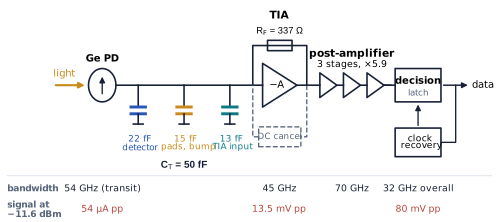
figsrc/ch21_rx.py.Step 1 · Turn the specification into a noise budget. At 50 Gb/s a bit lasts 20 ps, one unit interval (UI). A BER of \(10^{-12}\) needs \(Q = 7.03\). The link budget of Chapter 33 assumes the sensitivity of Example 21.2, −11.6 dBm with a 4 dB extinction ratio (thermal, shot and dark-current noise included): 69.2 µW on average, an OMA of 59.6 µW, and so a photocurrent swing \(I_1 - I_0 = 53.6\) µA. With the same noise on both levels, \(I_1 - I_0 = 2Q\sigma\), so all the noise of the front end together, referred to its input, must stay below \(\sigma = 3.81\) µA rms. That one number is the budget every later step spends. The other end of the range matters too. The link actually delivers −2.7 dBm: 483 µA of average photocurrent and a 416 µA swing. That is 8.9 dB more light but 17.8 dB more electrical signal power, because the photocurrent is proportional to the optical power and electrical power to the square of the current [88]. The front end has to decide correctly over this whole dynamic range.
Step 2 · Count the capacitance. The photodiode of Worked Example 21.1 brings 17 fF of junction and 5 fF of wiring. In the reference link the TIA sits on a separate CMOS chip, flip-chipped onto the photonic chip, so two pads and a micro-bump add about 15 fF (an assumed value; wire bonds and ESD protection add more, and inductance as well). The TIA’s own input transistor adds \(C_I \approx g_m/2\pi f_T\): 12.7 fF for a transconductance of 16 mS in a process whose transistors reach \(f_T \approx 200\) GHz. The total, \(C_T \approx 50\) fF, is more than twice the photodiode’s own capacitance, and it sets almost everything that follows. Step 5 shows what it is worth: without the pads (a monolithic receiver, 35 fF) the sensitivity would be 1.4 dB better, and 40 fF more of wire-bond pads would cost 2.4 dB.
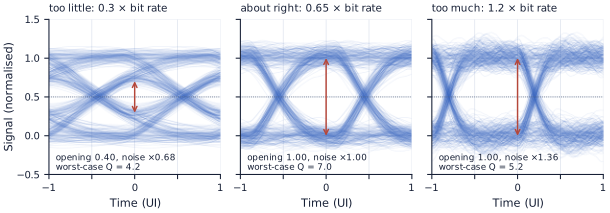
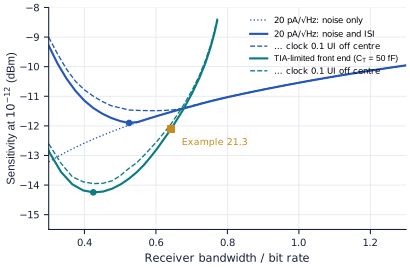
Step 3 · Choose the bandwidth. With too little bandwidth each bit’s response spills into the next, intersymbol interference (ISI), and the eye closes; with too much the receiver collects more noise for nothing. Figure 21.2 shows the eye at the decision circuit for three bandwidths of the same receiver at the same received power. For a noise density that does not change, the rms noise grows as the square root of the noise bandwidth (1.11 \(f_{3\mathrm{dB}}\) for this second-order response). At 0.3 times the bit rate the noise is 0.68 times smaller, but the worst-case eye has closed to 0.40 of its full height and Q falls from 7.0 to 4.2. At 1.2 times the bit rate the eye is fully open, but the noise is 1.36 times larger and Q is 5.2. Swept finely, this receiver needs the least power at about 0.53 times the bit rate, and at about 0.60 times if the clock may sample 0.1 UI away from the centre of the eye (Figure 21.4, blue). Hence the rule of thumb that a receiver’s bandwidth should be 0.5–0.7 times its bit rate [77].
figsrc/ch21_rx.py.The bandwidth that counts is that of the whole chain, photodiode included. For cascaded blocks the inverse squares of the bandwidths roughly add,
\[\frac{1}{f_{3\mathrm{dB}}^2} \approx \sum_i \frac{1}{f_i^2},\]so each block must be faster than the whole. The photodiode’s transit-time limit (54 GHz, Worked Example 21.1) is spent before the TIA. A 45 GHz TIA and a 70 GHz post-amplifier then give 31.0 GHz by this rule, and 32.1 GHz, 0.64 times the bit rate, when the cascade is computed exactly. That is the first-pass allocation: the TIA has to reach 45 GHz.
Step 4 · Pick the TIA. The simplest front end is a resistor: the photocurrent flows through \(R\), and the voltage across it is the signal. Its bandwidth is \(1/2\pi R C_T\), so 45 GHz with 50 fF allows only 71 Ω. That resistor’s thermal noise, \(\sqrt{4kT/R}\) = 15.3 pA/√Hz, is bad enough. Worse, a gain of 71 Ω leaves the signal so small that the next amplifier’s own noise (1.58 nV/√Hz, Step 5), referred back to the input, is 22 pA/√Hz. Over the same chain the total is 7.05 µA rms, nearly twice the budget.
The shunt-feedback TIA breaks this tie. An inverting amplifier of gain \(A\) with a resistor \(R_F\) from its output to its input holds the input almost still: the input resistance is \(R_F/(A+1)\), so the input pole moves out by \(A + 1\), while the transimpedance stays close to \(R_F\) (\(R_T = R_F A/(A+1)\)). If the amplifier were infinitely fast, \(f_{3\mathrm{dB}} = (A+1)/2\pi R_F C_T\), and the transimpedance for a given bandwidth would grow in proportion to \(A\). But the amplifier has its own pole, at \(f_A\), and its gain–bandwidth product \(A f_A\) is fixed by the process and the current it draws. With two poles the response is second order, and the largest transimpedance that still gives a flat (Butterworth) response is the transimpedance limit [91, 89]:
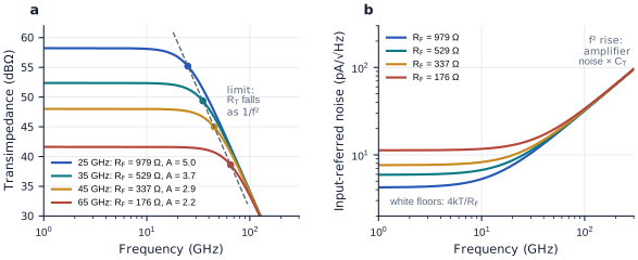
The bandwidth enters squared: for a given amplifier and input capacitance, twice the bandwidth costs four times the transimpedance. In CMOS the amplifier is usually an inverter. Its NMOS and PMOS transistors share one bias current and both contribute transconductance, and it works from a supply below a volt, where stacked circuits run out of headroom. Our inverter, 16 mS driving 16 fF, has a gain–bandwidth product of 159 GHz. With \(C_T\) = 50 fF and 45 GHz the limit is 252 Ω (48 dBΩ), reached with \(A = 2.9\) and \(R_F\) = 337 Ω. Figure 21.3a shows this design among others: a 25 GHz TIA could have 815 Ω, a 65 GHz one only 121 Ω. A gain of 2.9 is less than an inverter gives on its own; lowering it (to an output resistance \(A/g_m\) of 184 Ω) is what moves the amplifier’s pole out to the 54 GHz that the flat response needs.
Step 5 · Add up the noise. Two sources dominate inside the TIA. The feedback resistor adds a white current noise \(4kT/R_F\): 7.0 pA/√Hz for 337 Ω. The input transistor has a channel noise, a voltage \(4kT\Gamma/g_m\) at its input with \(\Gamma \approx 1\). The input current must charge \(C_T\) to follow that voltage, so referred to the input it becomes a current noise that rises with frequency:
The \(f^2\) part crosses the resistor’s floor at 22 GHz and reaches 10.2 pA/√Hz at the 32 GHz band edge (Figure 21.3b). To turn a spectrum into an rms noise, integrate it over the receiver’s response. Personick’s integrals package that integration: the white part is collected over a noise bandwidth \(I_2 B\) and the \(f^2\) part over \(I_3 B^3\), where \(I_2\) and \(I_3\) are numbers set only by the shape of the response [92, 77]. For a second-order Butterworth response at 0.7 times the bit rate, \(I_2 = 0.78\) and \(I_3 = 0.37\). The \(B^3\) is the point: at high bit rates the noise is set by \(C_T\) and \(g_m\) more than by \(R_F\). The post-amplifier adds its own input noise, 1.58 nV/√Hz from a 10 mS input pair, divided by \(R_T\): 6.3 pA/√Hz.
Integrated over the whole chain, the three parts give 1.43 µA (feedback resistor), 2.15 µA (amplifier) and 1.78 µA (post-amplifier). They add as squares, to 3.14 µA: inside the 3.81 µA budget, and equivalent to 16.8 pA/√Hz over Example 21.2’s 35 GHz. Every term depends on \(C_T\), which is why Step 2 mattered: with 35 fF the noise would be 2.29 µA, with 90 fF 5.39 µA.
Here is the central trade of the TIA. For a given amplifier and \(C_T\), a larger \(R_F\) lowers the resistor’s noise and puts more gain ahead of the post-amplifier’s noise, but lowers the bandwidth; a smaller \(R_F\) does the opposite. Transimpedance, bandwidth and noise cannot be chosen separately. Only more gain–bandwidth (more current, a faster process) or less capacitance improves all three at once.
figsrc/ch21_rx.py.Step 6 · Add gain: the post-amplifier and the decision circuit. At sensitivity the TIA’s output swings only 53.6 µA × 252 Ω = 13.5 mV. The decision circuit is a clocked latch that regenerates a small difference into full logic levels, but it has an offset and noise of its own; suppose it needs 80 mV to decide cleanly. The post-amplifier must then supply a gain of 5.9 (15.5 dB) with 70 GHz of bandwidth. One stage with the inverter’s 159 GHz gain–bandwidth product would reach only 27 GHz at that gain. Splitting the gain over \(n\) stages helps, because each stage’s bandwidth grows as its gain falls, while the bandwidth of \(n\) identical stages shrinks only by a factor \(\sqrt{2^{1/n} - 1}\) (0.51 for three). For the widest bandwidth each stage should have a gain of about \(\sqrt{e} \approx 1.65\), which here means \(2\ln 5.9 = 3.6\) stages [90]. Three plain stages of 1.81 each reach 45 GHz; to reach 70 GHz, each stage needs 1.56 times the gain–bandwidth product of a plain stage. Inductive peaking supplies that at no extra power: a small inductor in series with each load resistor extends a stage’s bandwidth by up to about 70 % before its response starts to peak [90]. At high input powers the last stages saturate; for NRZ that is harmless, and it gives the block its usual name, limiting amplifier. At −2.7 dBm the signal would otherwise reach 621 mV.
Two slow effects need loops of their own. The average photocurrent, 483 µA at −2.7 dBm, would shift the TIA’s output by 163 mV through \(R_F\). A slow DC-cancellation loop sinks it at the input, which also keeps the decision threshold in the middle of the eye whatever the received power. And any offset between the threshold and the centre of the eye costs sensitivity. An offset \(\Delta V\) on a swing \(v_\mathrm{pp}\) means that one level must move \(\Delta V\) further away, a penalty of \(10\log_{10}(1 + 2\Delta V/v_\mathrm{pp})\) [77]. With 80 mV at the latch, 1 mV of residual offset costs 0.11 dB and 3 mV costs 0.31 dB, so the post-amplifier carries an offset-cancellation loop as well. Both loops must be much slower than the longest run of identical bits, or they would remove the low-frequency content of the data. Finally, the latch’s own noise, 1 mV rms, divided by the total transimpedance from photocurrent to latch, 1492 Ω (63.5 dBΩ), adds 0.67 µA: 3.21 µA in all.
Step 7 · Check the eye and the sensitivity. Simulating the PRBS7 pattern through the whole chain gives an eye open to 0.998 of its full height at the best sampling instant (an ISI penalty of 0.01 dB), and to 0.960 when the clock samples 2 ps (0.1 UI) early or late. With the thermal noise, the photodiode’s shot and dark-current noise (as in Section 21.6), the latch’s noise and offset, and the ISI, the sensitivity is −12.1 dBm at \(10^{-12}\): 0.5 dB better than the −11.6 dBm the link budget assumes. Timing has a budget too: random jitter of the sampling clock, \(\sigma_\mathrm{RJ}\) rms, uses \(2Q\sigma_\mathrm{RJ}\) of the unit interval, so 0.3 ps rms already takes 4.2 ps of the 20 ps.
Step 8 · Count the power. The TIA itself is cheap. At a \(g_m/I_D\) of 8 V⁻¹ in each transistor, the inverter’s 16 mS needs 1.0 mA: 0.9 mW from 0.9 V. The three post-amplifier stages take 2.5 mA each, 6.75 mW, and the loops and biasing about 0.3 mW. The analogue front end therefore uses about 8 mW, 0.16 pJ/bit at 50 Gb/s. Table 33.1 budgets 1.0 pJ/bit, 50 mW per lane, for the receivers. That leaves about 42 mW for the latches, clock recovery, deserialiser and output drivers, which in practice take most of a receiver’s power.
- Specification. 50 Gb/s NRZ at \(10^{-12}\) (\(Q = 7.03\)) and −11.6 dBm with 4 dB extinction: a 53.6 µA swing, so at most 3.81 µA rms of input-referred noise.
- Capacitance. 22 fF photodiode + 15 fF pads and bump + 12.7 fF TIA input = 50 fF.
- Bandwidth. About 0.6 times the bit rate overall. With the photodiode’s 54 GHz, the TIA gets 45 GHz and the post-amplifier 70 GHz: 32.1 GHz overall.
- TIA. An inverter core with a gain–bandwidth product of 159 GHz; the limit allows \(R_T\) = 252 Ω at 45 GHz, with \(A\) = 2.9 and \(R_F\) = 337 Ω.
- Noise. 1.43 µA (feedback resistor), 2.15 µA (amplifier) and 1.78 µA (post-amplifier), added as squares: 3.14 µA, and 3.21 µA with the latch.
- Gain. Three peaked stages, × 5.9 in all, take 13.5 mV to 80 mV: 1492 Ω from photocurrent to latch.
- Eye and sensitivity. The eye is 0.998 open (0.960 with the clock 2 ps off centre); the sensitivity is −12.1 dBm, 0.5 dB better than assumed.
- Power. 0.9 mW in the TIA, 6.75 mW in the post-amplifier and 0.3 mW in the loops: about 8 mW, 0.16 pJ/bit.
21.9Equalisation, clock recovery and measuring sensitivity
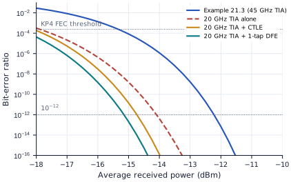
A narrower TIA is quieter. Step 3 assumed a noise density that does not change with bandwidth. A TIA’s does. The transimpedance limit forces \(R_F\) down as \(1/f_{3\mathrm{dB}}^2\), which raises its \(4kT/R_F\) noise; the lower transimpedance lets more of the post-amplifier’s noise through; and the \(f^2\) noise integrates to \(B^3\). Going from a 30 GHz to the 45 GHz TIA of Example 21.3 widens the whole receiver by 28 % (from 25.1 to 32.1 GHz) but raises the noise by 79 % (from 1.76 to 3.14 µA): the noise grows roughly as the bandwidth to the power 2.4, not 0.5. Figure 21.4 repeats the bandwidth sweep of Step 3 with this front end. Its best sensitivity, −14.25 dBm, now comes at 0.43 times the bit rate (a 24 GHz TIA), 2.1 dB better than Example 21.3. With a TIA-limited front end it pays to make the TIA slower than the classic rule suggests and then to repair the ISI. Many recent receivers do exactly that, some with a TIA bandwidth well below half the symbol rate [89, 82].
figsrc/ch21_rx.py.Equalisers. Take a TIA of only 20 GHz (\(A\) = 6.1, \(R_F\) = 1482 Ω, \(R_T\) = 1273 Ω). Its noise is just 0.99 µA, but the whole receiver’s bandwidth falls to 18.3 GHz (0.37 times the bit rate) and the worst-case eye to 0.60 of its full height. Even so it reaches −14.0 dBm, because the noise it saves outweighs the ISI it causes. Two kinds of equaliser win back part of the eye [77, 89]:
- A continuous-time linear equaliser (CTLE) is a filter with a zero and a higher pole, which lifts the high frequencies that the TIA has cut. One with a zero at 16 GHz and a pole at 35 GHz (6.8 dB of boost) restores 24.9 GHz of bandwidth and opens the eye to 0.91. But it lifts the high-frequency noise along with the signal, to 1.51 µA: −14.5 dBm.
- A decision-feedback equaliser (DFE) subtracts the ISI that the previous bits leave in the present one. It knows those bits because it has just decided them, so the subtraction adds no noise. Here the previous bit leaves 0.18 of the full step in the present one (whose own share, the main cursor, is 0.82). A one-tap DFE removes it and opens the eye to 0.76 with the noise unchanged: −15.0 dBm, 2.9 dB better than Example 21.3, and −15.2 dBm with two taps.
The DFE has costs that these numbers hide. It cannot remove pre-cursor ISI, from bits not yet decided; a feed-forward equaliser, often in the transmitter, does that. Its first tap must be decided and subtracted within one unit interval, 20 ps, so designs compute both possible corrections in advance and let the previous bit choose between them (loop unrolling). A wrong decision feeds back a wrong correction, but at low BER such error propagation is rare. The tap weights adapt in the background, typically through a sign–sign LMS loop fed by extra samplers with offset thresholds. A narrow, high-\(R_F\) TIA also overloads sooner: at −2.7 dBm this one would swing 530 mV, with 716 mV of DC across \(R_F\), so it needs the DC-cancellation loop and an automatic gain control that lowers \(R_F\) for strong signals. Equalisers also repair ISI that does not come from the receiver: if the transmitter’s ring modulator (Chapter 20) behaved like a single 35 GHz pole (an assumed value), Example 21.3 would lose 0.66 dB and the DFE receiver 0.47 dB.
figsrc/ch21_rx.py.Clock and data recovery. No clock travels with the data, so the receiver recovers one from the data’s own transitions. A phase detector compares each transition with the clock and reports early or late, a loop filter averages the reports, and an oscillator or phase interpolator moves the clock until the transitions fall midway between sampling instants, which puts the samples in the middle of the eye. The loop is slow (megahertz, not gigahertz), so it follows slow wander of the data’s phase but not fast jitter. At 50 Gb/s the latches are usually clocked at a half or a quarter of the bit rate on interleaved phases (four phases of a 12.5 GHz clock), which also demultiplexes the data into slower lanes. The timing budget is the horizontal counterpart of Q [77]. Deterministic jitter (DJ, from ISI, duty-cycle error and crosstalk) adds linearly; random jitter is multiplied by \(2Q\):
\[\mathrm{UI} \ge \mathrm{DJ} + 2Q\,\sigma_\mathrm{RJ}\]A bathtub curve, the BER against sampling phase, measures the remaining timing margin directly.
Measuring sensitivity. A pattern generator drives a reference transmitter of known extinction ratio; a variable optical attenuator sets the received power, monitored through a tap and a power meter; an error detector compares the recovered bits with the pattern. Stepping the power traces a waterfall curve like those of Figure 21.5. Measuring \(10^{-12}\) directly is slow: seeing no errors in \(3.0\times10^{12}\) bits gives 95 % confidence that the BER is below \(10^{-12}\), which takes 60 s at 50 Gb/s for every power, against 60 ms for \(10^{-9}\). So the curve is usually measured at higher BERs and extrapolated. For a receiver limited by thermal noise, Q is proportional to the received power, so \(10\log_{10}Q\) against power in dBm is a straight line of slope 1, and a few points between \(10^{-5}\) and \(10^{-9}\) fix where it crosses \(Q = 7.03\) [77]. A link that runs KP4 FEC is tested at the threshold, \(2.4\times10^{-4}\), in a fraction of a second. Quoting the sensitivity as an OMA makes it independent of the test transmitter’s extinction ratio. Standards also specify a stressed sensitivity, measured with a deliberately degraded input eye (added ISI, jitter and noise), so that a receiver proves its margin against a realistic transmitter rather than a perfect one.
Waveguide-coupled vertical Ge PIN photodiodes (about 15 × 4 µm, 0.5 µm intrinsic, about 0.9 A/W and 48 GHz) on each drop port, each with a TIA of about 20 pA/√Hz. Sensitivity about −11.6 dBm at BER 10⁻¹² (−14.7 dBm with KP4 FEC). Monitor taps on the drop rings’ through ports feed the locking loops. Front end (Worked Example 21.3): about 50 fF at the input with flip-chip bonding, a 45 GHz inverter TIA with \(R_F \approx\) 340 Ω, a three-stage peaked post-amplifier, about 8 mW per lane; −12.1 dBm, so the budget’s −11.6 dBm holds with 0.5 dB in hand. A 20 GHz TIA with a one-tap DFE would gain about 3 dB more.
Reading
- [37] Jurgen Michel, Jifeng Liu and Lionel C. Kimerling. “High-performance Ge-on-Si photodetectors.” Nature Photonics, 4:527–534, 2010.
- [73] Jifeng Liu, Jurgen Michel et al. “High-performance, tensile-strained Ge p-i-n photodetectors on a Si platform.” Applied Physics Letters, 87:103501, 2005.
- [1] Lukas Chrostowski and Michael Hochberg. Silicon Photonics Design: From Devices to Systems. Cambridge University Press, 2015. https://www.cambridge.org/core/books/silicon-photonics-design/BF3CF13E8542BCE67FD2BBC7104ECEAB
- [74] Eduard Säckinger. Broadband Circuits for Optical Fiber Communication. Wiley-Interscience, 2005.
- [77] Sam Palermo. “Lecture 4: Receiver Analysis.” ECEN 721: Optical Interconnects Circuits and Systems, Texas A&M University, Spring 2026. https://people.engr.tamu.edu/spalermo/ecen689_oi/lecture4_ee721_rx_analysis.pdf
- [89] Sam Palermo. “Lecture 5: Transimpedance Amplifiers (TIAs).” ECEN 721: Optical Interconnects Circuits and Systems, Texas A&M University, Spring 2026. https://people.engr.tamu.edu/spalermo/ecen689_oi/lecture5_ee721_tias.pdf
- [90] Sam Palermo. “Lecture 6: Limiting Amplifiers (LAs).” ECEN 721: Optical Interconnects Circuits and Systems, Texas A&M University, Spring 2026. https://people.engr.tamu.edu/spalermo/ecen689_oi/lecture6_ee721_limiting_amps.pdf
- Responsivity is η λ[µm]/1.24 A/W: at most 1.25 A/W at 1550 nm. Germanium on silicon, tensile-strained, absorbs across the C band.
- Waveguide-coupled photodiodes absorb along their length, so they can be thin, fast and efficient at once; normal-incidence ones trade responsivity for speed.
- The bandwidth combines the transit limit (0.45 vsat/d) and the RC limit: about 48 GHz for a 15 × 4 µm, 0.5 µm detector.
- TIA thermal noise dominates short-reach receivers. BER = ½ erfc(Q/√2), with Q = 7.03 for 10⁻¹² and 3.49 for the KP4 FEC threshold.
- The reference-link receiver needs about −11.6 dBm at 10⁻¹² with 4 dB extinction, leaving about 9 dB of margin; APDs and FEC buy several decibels more.
- Design a front end from its noise budget: at −11.6 dBm, 4 dB extinction and 10⁻¹², at most 3.8 µA rms at the input. About 50 fF of input capacitance (photodiode, pads, TIA input) shapes everything after it.
- A shunt-feedback TIA’s transimpedance is limited to A fA/(2π CT f²): 252 Ω at 45 GHz here. Its noise is 4kT/RF plus an f² term from the amplifier acting through CT. Worked Example 21.3 reaches 3.1 µA rms and −12.1 dBm for about 8 mW (0.16 pJ/bit).
- With constant noise density the best receiver bandwidth is 0.5–0.7 times the bit rate; a TIA-limited front end’s noise grows about as bandwidth2.4, so a narrower TIA with a DFE gains about 3 dB.
- Clock recovery keeps the sample in the centre of the eye; random jitter costs 2Qσ of the unit interval. Proving 10⁻¹² takes 60 s at 50 Gb/s, so sensitivity is usually extrapolated from higher BERs.